This is my research diary about intelligence in 2019. I find writing research diary really interesting and it helps me to organize my thougths and discover new ideas! I just hope I have enough thougths to continue writing.

Reference

January

01/21: What is intelligence? (1/2)

I’m going to talk about intelligence. To be specific, it is not just human intelligence or artificial intelligence but general intelligence that I want to talk about. Although it is really hard to find a proper and satisfying defnition for intelligence, it is still possible to name some traits of intelligence. Let’s begin!

Adaptive: Intelligence is adaptive and flexible, easy to adjust itself. It should have a strong adaptivity that enables it to adapt to any environments. Image that a baby born on Mars or Moon. Although the gravaity is different than it on Earth, it won’t take the baby too long to get used to the new environment. For human being or other forms of life, this ability is essential to their survival. So it is for an intelligent agent. Afterall, an agent that fails to survive cannot have enought time to do what it needs to do.
But what does this abstract word, adaptive, really mean? Well, it is about making right decisions. But what is right? And how to make right descisions? Since I don’t have a clear answer rigt now, it is better to leave it for future elaboration.
Robust: An intelligent agent should be complex enough to cope with possible errors. There are basic two ways: the self-correcting way and the fault-tolerant way. The self-correcting way is more active while the fault-tolerant way is more passive. Robustness overlaps with self-optimizing (see below).
Self-optimizing: While making actions is about changing the outside state, self-optimizing is about changing the inner state of the agent itself. Self-improving is a simliar word. Evolving has a broader meaning. It emphasizes changing, not just improving or optimizing. Updating knowledge system and optimizing action outputs are two good examples. In a word, the agent improves itself in order to better achieve the goal.

Note that the three traits mentioned above are strongly connect with each other.

01/22: What is intelligence? (2/2)

Efficient: In real world, we often need to solve optimzation problems, such as finding the shortest way to school, makeing as much as money given fixed time and being sucessful as young as possible. In short, we want to achieve the goal efficiently. Similarly, a good intelligent agent should be efficient enough to realize the final goal. For example, energy saving and less time wasting. However, this may not always be the case because I am talking about efficiency in the sense of archieving goal. The goal can also be related to inefficiency, such as riding a bike as slow as you can. So the efficiency I mean, is based on the goal totally. Planning and optimization play important roles here.
Learning ability: Although by hardcoding knowledge into an agent’s “brain” may solve most practical problems, it requres a great amount of manual work. Moreover, it is not flexiable——hardcoding means it is not easy to update current knowledge thus making self-optimizing impossible.
Instead of trying to produce a programme to simulate the adult mind, why not rather try to produce one which simulates the child’s? (Alan Turing) Children have incredible learning ability and they learn fast. They are born with the ability to learn which is encoded in DNA during the long period of evolution.
Life long learning, few shot learning, multi-task learning, multi-agent Learning, meta learning and transfer learning can all be included in this part. Next, I will introduce two aspects of learning:
- learning knowledge: This is the most obvious aspect of learning. It is a process of extracting features, patterns and rules from raw data generated by the interaction between the agent and the environment (direct experience) or from existing data (indirect experience). It’s similar to discovery of physics laws. Supervise and unsupervise learning are two good examples. Moreover, after discovering new knowledge, it is also necessary to embed it into current knowledge system and to make connections from old knowledge to new knowledge. By doing this, an agent can accumulate knowledge as time goes on and wield knowledge in a more powerful way. Finally, the agent is able to construct a model of the world.
  Is learning knowledge an application of funtion approximation? Can any knowledge be expressed as functions? To answer these questions, we need to define knowledge itself. Generally, what we call knowledge can be divided into two subgroups: the knowledge to environment and meta knowledge (the knowledge of knowledge itself). I leave it for future consideration.
- learning how to learn (also known as meta learning): Learning is not only about learning knowledge but also learning how to learn. I call this kind of knowledge as meta knowledge (the knowledge of knowledge itself). It is more abstract than the knowledge of environment, similar to (but not the same as) the relation between physics and mathematics (This is still not a good comparsion, but the best I can find right now.). Things like how to discover knowledge more quickly and when/where/how to apply it are two examples.
Others: creativity, imagination… The meaning of these words are vague and abstract. I don’t know how to translate them into more concrete ones. Maybe they are just manifestations of searching, exploring and combining old things into new things.

01/23: What’s inside in an intelligent agent?

The traits of intelligence are like softwares in a computer. So what hardwares do we need in order to support the normal running of softwares? In my opinion, these subsystems are necessary for an intelligent agent:

Sensor: Any things that preceives the environment counts as a sensor. An agent may have many sensors. A sensor can be defined as a mapping from environment to signals. For example, an ear transforms sound waves to acoustical signals and an eye transforms photons of lights to images. The sensors create what the agent can “see”. The signals that sensors output are the only information source of the environment. Anything that cannnot be perceived by sensors does not exist with regard to the agent. Note that what sensors perceive may be wrong, i.e. the signals produced by sensors do not reflect the real world accurately.
Actor: An actor is anything that an agent can control to influence the outside environment. It receives commands from the decision make and then act according to the commands appropriately. The actions include simple reflex action, model-based action and goal-based action. They can be atomic, factored or structured.
Decision maker: It is the brain of an agent and also the most important subsystem for decision making. The inputs are the signals received by sensors. And it outputs commands which are excuted by actors. To analyze it meticulously, I divide it into several parts.
- Knowledge base: A knowledge base is where an agent stores knowledge.
- Thinker: It is the core of descision maker and also employs most computation resources. It makes a series of decisions given access to knowledge base and signals from sensors. If necessary, it also updates knowledge in the knowledge base or even create a new one from scatch. It is the basis of intelligence. All other parts only exist to support it. I don’t have too many ideas about it and may spend the rest of my life to figure out how to make one.

Can we separate the knowledge base with the thinker totally? Yes! One good example is McCarthy’s Advice Taker in which the rules and the reasoning component are separated. But is it good? I’m not sure. It’s possible that these subsystems are strongly connected or even merged together without clear boundaries. If the knowledge base and the planner are separated completely, it may take more time to access necessary knowledge before making a proper decision. Thus, a distributed knowledge base may be more efficient. For example, knowledge in neural networks is represented by weight matrice between layers. The decision making process consists of repetitions of acessing to knowledge (weights) and computation (compute activation functions, do matrix multiplication, etc.). The two procedures are followed one after the other in the forward process. Further thoughts and emprical experiments are still needed.

01/24: Knowledge base

Before considering the knowledge base, it is better starting from more basic questions.

What avaliable knowledge representations we can use?
- Human language (written language): Almost any knowledge can be expressed as language. It has inner structures, mapping from symbols to real world objects or even from symbols to symbols, full of bootstraping and self-reference. It evolves as time goes.
- Vector: Methods such as word embedding, map words or phrases to vectors of real numbers. Since we can encode human language into a sequence of bytes (i.e. numbers) under some standard rules, any knowledge represented by human language can also be represented by a bunch of numbers (i.e. vectors). Afterall, they are all symbols.
- Graph: Knowledge graphs are human understandable and easy for computers to operate. They are also very powerful to represent knowledge. Maybe it can be a good interlanguage between human and computers. I don’t know too much about this. Need future study.
What is a good knowledge representation?
In fact, whether a knowledge representation is good or bad really depends on the agent itself and the goal. I should say that any knowledge that helps the agent to achieve the goal is a good one. Although it is hard to give a clear answer, typically, a good knowledge representation is:
- powerful: It should be able to express enough knowledge.
- compact: The representation should have high information density which is space-saving.
- easy to operate: It should be easy to handle and operate by the agent.
  
  Note that a good representation is not necessary human readable although it will be really helpful.
Now let’s consider knowledge base. A good knowledge base is:
- easy to retrive: It should be easy (less time consuming) for agent to find necessary knowledge.
- easy to update: It should be easy to add, delete and change knowledge in the database.
- space-saving: If the knowledge is too small, then there will not be enough space to store all knowledge the agent discovers. However, if it is too big, it takes a large amount of time to access. Both cases are not favourable. The best way to resolve this conflict is to find a space-saving way to store knowledge. Some compression methods can be applied if it is necessary, suitable and appropriate.
How do we (i.e. human being) store and retrieve memory? No idea. Need future study.

01/25: Reward function (1/3)

How to guide an agent to achieve the final goal. Use reward! (But do we really need it? Is it necessary?)

Are binary ((0,1),(-1, +1)) or integer reward functions as powerful as any real number reward functions?
“Powerful” is not very clear. What I mean is that can any policy generated using real number reward functions be generated by binary reward functions? I think the answer should be “Yes”. In general value iteration, we first do policy evaluation by computing state values or state-action values based on reward sequence we receive. After that, policy improvement is applied to find better policies. To be more specific, we need the information about how to choose the best action given state values or state-action values. How do we do this? We compare numbers and then choose the action with max state-action value. In fact, it doesn’t matter whether these numbers are real numbers or integers. What matters is the order. And integer is an ordered field which should be enough. However, real reward function has a big advantage. Since real number field is dense, we can always find a real number between two different real numbers. For example, asumme that we assign $1$ to $Q(s,a _ 1)$ and $2$ to $Q(s,a _ 2)$. Then here comes $Q(s,a _ 3)$. And we find that $a _ 3$ is better than $a _ 1$ but worse than $a _ 2$, i.e. $1=Q(s,a _ 1) < Q(s,a _ 3) < Q(s,a _ 2)=2$. We can always find a real number between 1 and 2 for $Q(s,a _ 3)$ but not an integer. If we insist to use integers, we must adjust the value of $Q(s,a _ 1)$ and $Q(s,a _ 2)$ as well. So apparently, real number reward functions are easier to use. But binary and integer reward functions have their own merits——they are easier to design. Which one is more sample efficient? Which one helps the agent learn faster? Need future study.

01/26: Reward function (2/3)

What are we talking about when we talk about rewards?

What are rewards? Where do they come from? Look around and then you will find that there are many things that we call reward, such as money paid by your boss, delicious food, compliment from people who respect you. But are they really reward? Definitely not! They are just what they are. We create rewards ourselves. Rewards come from our brain, especially the chemical reward system in the brain. Through the chemical reward system, the brain guides the body, drive it for food and away from danger. In short, rewards are interpretations of current state (both the environment and agent itself). They are a measure how good or better the current state is. And how close are we from the final goal. Typically, we use a real number to indicate this. The larger the reward value is, the better the current state is and the closer we are from the final goal. For example, if the goal is finding the shortest path from $cityA$ to $cityB$, the reward can be the inverse of path length from current position to $cityB$.

Note that the reward I’m talking about here is not same as the reward descriped in Reinforcement Learning. The reward in RL defines the goal, indicates what is good or bad in an immediate sense. In this context, however, it indicates what is good or bad in the long run. So for consistency, I call the reward that I mentioned before cumulation, denoted as $C_t$ at time $t$. And the new reward $R_t$ is defined as a function of cumulation, i.e. $R _ t \doteq C _ t - C _ {t-1}$. In another view, the cumulation is a cumulative sum of the reward sequence: $C _ t = R _ 1 + R _ 2 + \cdots + R _ t = \sum _ { k = 1 } ^ { t } R _ { k }$. The new reward is same as the reward in RL. But the cumulaiton is not return. As a reminder, the return is defined as $G _ { t } \doteq R _ { t + 1 } + R _ { t + 2 } + R _ { t + 3 } + \cdots + R _ { T }$. The return is a accumulation of future rewards while cumulation is a accumulation of past rewards. They are two aspects.

Similar to discounted return, we can also add discount factor to cumulation: $C _ t = R _ 1 + \gamma R _ 2 + \cdots + {\gamma} ^ {t-1} R _ t = \sum _ { k = 1 } ^ { t } \gamma ^ { k - 1 } R _ { k }$ and $R _ t = \frac{C _ t - C _ {t-1}}{{\gamma} ^ {t-1}}$.

01/28: Reward function (3/3)

As I elaborated in last research diary, “Rewards are interpretations of current state (both the environment and agent itself). They are a measure how good or better the current state is. And how close are we from the final goal.” So $R _ t$ should be a function of environment state $s _ {env}$ and agent state $s _ {agent}$, i.e. $R _ t: S _ E \times S _ A \rightarrow \mathbb{R}$ where $S _ E$ is the environment state space and $S _ A$ is agent state space. In current typical RL setting, $R _ t$ is only determined by the environment. The agent state is not considered. This is because first, the reward design remains to be a difficult problem. Second, most RL agents are too simple. There are no such thing as agent states!

Instead of designning reward functions manually, can we design some methods to learn reward functions? For example, can we apply neural networks to approximate the true rewards (if they do exist) through bootstrapping? I think there should be some previous works (It’s so obvous afterall!), or maybe someone tries this idea before but it didn’t work. Need future study.

The agent–environment interaction in a MDP.

01/29: State

Define the state space $S$ to be $S \doteq S _ E \times S _ A$ where $S _ E$ is the environment state space and $S _ A$ is the agent state space. For every state $s$, it can written as $s=(s _ e, s _ a)$. If we use a vector to represent a state $s$, then each dimension of this vector is a feature of this state (e.g. $s=(f _ 1, f _ 2, \cdots, f _ n)$).

One advantage of representing states using vectors is that vectors are simple, comprehensible and easy to handle—they are just a bunch of features. However, since there is no internal structure inside a vector, it is not convenient to represent complex states or encode structural information in it, such as feature interaction (e.g. ${f _ 1 ^ 2} f _ 2$). One way to fix this is adding new features (e.g. $f _ {n+1} = {f _ 1 ^ 2} f _ 2$). But this usually leads to the curse of dimensionality. Thus we need a more compact but still powerful enough representation. And they should be manageable by agents (e.g. computers).

How about structural representations, such as trees and graphs? Are they good representations for states? Well, I’m not sure. Take the graph for example. If nodes are objects or features, edges that connect nodes can be the relations between objects or features. They are more powerful than vectors, since ordered disconnected nodes are equivalent to vectors. Moreover, nodes may have inner structure. In fact, we can even include part of graph inside a node! However, since graphs are more complex than vectors, they are also more difficult to handle with. And what is the edge that connects two nodes in the sense of mathematics? Need future study.

01/30: Action (1/2)

Let $A$ be the action space. Then an action can be viewed as a mappings from a distribution of state space to another distribution of state space, i.e. $A: p(S) \rightarrow p(S)$. Note that this includes the mappings from one state to another state if all probability is concentrate on a particular state, i.e. $p(s)=1$ for state $s$ while $p(\cdot)=0$ for other states. For example, $a(p _ 1)=p _ 2$ where $p _ 1(s)=\mathcal{N}(0,1)$ and $p _ 2(s)=\mathcal{N}(1,4)$.

If an action only influences the variation between two distributions, we have following properties:

$\Delta {p _ a} \doteq p _ 1 - p _ 2$ is only determined by action $a$ where $a(p _ 1)=p _ 2$. To be specific, $p _ 2 \doteq a(p _ 1)=p _ 1 + \Delta {p _ a}$.
$\int_{s \in S} \Delta {p _ a} ds = 0$

Note that this is still not well-defined. For example, $\Delta {p _ a}(s) = s$ for $s \in S=[-1,1]$. $p _ 1$ is a uniform distribution, defined as $p _ 1(s) = 1/2$. Then $p _ 2 \doteq a(p _ 1) = p _ 1 + \Delta {p _ a} = s + 1/2$. Easy to see $p _ 2 (s=-1) = -1/2$. However, $p _ 2$ is a probability density function, so $p _ 2 (s) \geq 0$ for all $s \in S$.

A possible way to fix this: we move the distribution function by a constant $c$, i.e. $p(s) =p(s) + c$ such that $\int_{s \in S} {max(p(s)+c, 0)} ds = 1$. The $p _ 2$ in the above example then becomes $p _ 2(s) = s + \sqrt{2} - 1$ for $s \in [1 - \sqrt{2}, 1]$ . This is not a good solution since the computation of $c$ is not easy.

However, if we use sampling, a negative probability won’t be a big problem. We can always sample from states that have a positive probability and discard the state we sampled out whose probability is negative.

February

02/01: Action (2/2)

Recall that $p(s ^ { \prime } | s , a)$ is the probability of transition from state $s$ to $s ^ {\prime}$ under action $a$. We also have: $$p _ 2(s ^ {\prime})= \sum_{s \in S} p(s ^ { \prime } | s , a) p _ 1(s) \quad \textrm{where} \quad a(p _ 1) = p _ 2$$

However, we can not recover state transition probability $p(s ^ { \prime } | s , a)$ simply from $p _ 1(s)$ and $p _ 2(s)$ since there are more unknown values than equations. This means that we can not have all information from $a(\cdot)$. But is $a(\cdot)$ useful enough? I don’t know actually…

We divide all actions based on state space $S$ roughly in three categories:

Atomic actions: They have no internal structures and are indivisible. They are the lowest level actions an agent can act. They are simple but also important. They are the points in the action space $A$. For completeness, we also add the identity action $a _ I$ in $A$ where $a _ I(p)=p$ for all $p$.
Composite actions: They are the actions in $A ^ n$ where $n \in \mathbb{N}$. For each composite action $a$, it is defined as $a \doteq a _ 1 \circ \dots \circ a _ n$ where $a _ i \in A$ for all $i \in {1, 2, \dots ,n}$.
Total actions: They are all possible actions that th agent can use, denote as $A ^ \infty$. For each action $a \in {A ^ \infty}$, it is defined as $a \doteq a _ 1 \circ a _ 2 \circ \dots \circ \dots = \circ _ {i=1} ^ {\infty} a _ i$ where $a _ i \in A$ for all $i \in \mathbb{N}$.

02/02: Hierarchical states and actions

Hierarchical states and actions are quite useful in planning and solving other problems. One way of constructing hierarchical states is abstraction (any other ways?). Then the natural questions are: what is abstraction and how to do that?

Well, abstraction is about leaving out unnecessary details, focusing on only general characteristics. Instances that have the same abstraction should share something in common. Based on this idea, we define a abstract state set: $$AS_f \doteq [x \in \Omega | f(x) \in P ]$$ (There is a problem with the display of {}, I use [] instead.) where $\Omega$ is a set of instances; $f$ is a transform function that the abstract state set bonds to; $P$ is a set that represents some properties. For example, $\Omega = \mathbb{R} ^ n$; $f: \mathbb{R} ^ n \rightarrow \mathbb{R} ^ m$ is a projection function: $f(x) = y$ where $x=(v _ 1,\cdots,v _ n)$ and $x=(v _ 1,\cdots,v _ m)$, $m<n$; $P=[x=(v _ 1,\cdots,v _ m) \in \mathbb{R} ^ m | v _ 1 = \cdots = v _ m ]$. Under this setting, $AS_f = [x=(v _ 1,\cdots,v _ n) \in \mathbb{R} ^ n | v _ 1 = \cdots = v _ m ]$.

Tile coding and state aggregation are two ways of defining abstract state set. Perhaps a more specific and simple way of defining abstract state set is clustering. The idea behind is very simple: instances that near each other under some metric should belong to a same abstract class. This can be viewed as doing clustering in the instance space.

Moreover, we can continue to define the second level abstract state set based on the (first) abstract state set: $$AS _ {f} ^ {2} \doteq [x \in \Omega | f(x) \in P ]$$ where $\Omega$ is a subset of $AS _ {g}$. Similarly, we can define $n$-th level abstract state set $AS _ {f} ^ {n}$.

Similar to how we define the action on state space, we can define the $n$-th level action on the $n$-th abstract state set.

02/04: Model (1/2): What is a model?

What is a model? According to Collins dictionary, “A model of an object is a physical representation that shows what it looks like or how it works. The model is often smaller than the object it represents.” In this definition, there are two important aspects:

The model is often smaller than the object it represents.
The model help us understand how the object looks like or how it works. Furthermore, the model helps us predict the behavior of the object.

What mathematical tools should we use to represent a model? Well, right now, for discrete process, we have deterministic finite automaton (DFA), nondeterministic finite automaton (NFA) and Markov decision process (MDP). In fact, they are quite similar. For continuous case, I don’t know too much yet. Need future study. So for the rest, I focus only on discrete case.

Based on MDP, I define a simliar but also different mathematical framework, called Markov transition process (MTP):

A MTP is a 5-tuple ($S, A, P _ a, S _ 0, F$), where

$S$ is a finite set of states.
$A$ is a finite set of actions.
$P _ {a}$ is the state transition probability defined as $a(p _ 1)=p _ 2$ for each action $a \in A$. If $p _ 1 (s) = 1$ for an action $a$, then we have $p _ 2 (s ^ {\prime}) = P _ {a} (s _ {t+1}=s ^ {\prime} \mid s _ {t}=s) = \operatorname{Pr}(s _ {t+1}=s ^ {\prime} \mid s _ {t}=s, a _ t = a)$ which is the probability that action $a$ in state $s$ at time $t$ will lead to state $s ^ {\prime}$ at time $t+1$.
$S _ 0 \subset S$ is a set of start states.
$F \subset S$ is a set of goal states.

Note that the hierarchical states and actions also fits the definition of MTP simply by replacing $Q$ and $A _ s$ whith $n$-th level abstract state set and $n$-th level action set, respectively.

Also, sometimes we need to model a world without the interference of the agent. We can include this case by adding null action denoted as $\emptyset$. Thus $P _ {\emptyset}$ the state transition probability for null action.

02/05: Model (2/2): Rethink

Things I need to consider further:

The above model is still too simple. Afterall, the world is not Markov.
The world is changing and evolving eternally. How can the above model deal with a changing world? How to update?
The world is so complex and there are so many possible states and actions. Thus it is impossible to store all state transition probability. Possible solutions：
1. Use function approximation.
2. Only save the most useful/important/relevent/latest state transition probability. Introduce forgetting mechanism.
3. Instead of saving a probability distribution, we save several next states with large probability.
Sometimes we don’t know the true state transition probability but only transition samples. Thus we need to calculate the estimated state transtion probability from samples. However, since all estimation is inaccurate and induce variance. How to resolve this problem without getting more samples?
How can we apply transfer learning or one-shot learning to new states transitions?
How do I predict the world? Do I have a world model in my brain? Do I store a set of states somewhere in my brain? If so, how does the brain represent a state?
How much information can we store in our brain in all our lives?

02/07: Policy (1/2)

According the definition in Sutton’s book, a policy defines the learning agent’s way of behaving at a given time; a mapping from perceived states of the environment to actions to be taken when in those states.

In RL setting, typically there are two ways to learn a policy:

Value-based methods: These methods (such as state value methods and state-action value methods) learn the action values and then select actions based on the estimated action values.
Policy gradient methods: Instead of estimating action values, these methods learn a parameterized policy that select actions without a value function. A value function may still be used to learn the policy parameter, but is not required for action selection (Sutton, 2018).

My question is that are there any other approaches to generate a policy? For example, rule-based methods? Futhermore, do we have to use a reward fucntion? Is it really necessary?

Instead, can we learn a metric $M$ that measures how “close” is the current state to the goal states? If so, then what supervised information can we use to correct a wrong measurement? But is this method really different with value-based methods? Maybe not.

02/08: Policy (2/2)

Anyway, let’s try! Define the metric over (abstract) state set: $M: S \times S arrow [0,+\infty)$. Since it is a metric, for $x,y,z \in S$, the following conditions are satisfied:

non-negativity: $M(x,y) \geq 0$
identity of indiscernibles: $M(x, y)=0 \Leftrightarrow x=y$
symmetry: $M(x,y)=M(y,x)$
Delta inequality: $M(x,z) \leq M(x,y) + M(y,z)$

We also have $M(F, F)=0$. Our goal is to reach a state $s$ such that $s= \arg \min _ {s \in S} M(s,F)$. Denote $\operatorname{Pr}(s _ {t+1}=s ^ {\prime} \mid s _ {t}=s, a _ t = a)$ as $\operatorname{Pr}(s ^ {\prime} \mid s, a)$ for short. Then for greedy action selection: $$\pi (s)=\arg \min _ {a \in A} \Sigma _ {s ^ {\prime} \in S} \operatorname{Pr}(s ^ {\prime} \mid s, a) M(s ^ {\prime}, F)$$ or more generally: $$\pi (s)=\arg \min _ {a \in A} \Sigma _ {s ^ {\prime} \in S} p _ 2(s ^ {\prime}) M(s ^ {\prime}, F) \text{ where } a(p _ 1)=p _ 2$$ Compared with value-based policy, $$ \pi (s)=\arg \max _ {a \in A} Q(s, a) = \arg \max _ {a \in A} \Sigma _ {s ^ {\prime} \in S} \operatorname{Pr}(s ^ {\prime} \mid s, a) (R + \gamma V(s ^ {\prime})) $$ notice that if $M(s ^ {\prime}, F) \propto -(R + \gamma V(s ^ {\prime}))$, the two ways of generating policy are exact same. So it seems that we still need use something similar to reward or state value as a measurement of the agent’s performance… Maybe this can be combined with some heuristic search algorithm or used as a better initilization for state values.

02/11: Transfer Learning: Introduction (1)

I’ve run out of my ideas. Time to learn new things. I start with transfer learning. After that, I’d probably continue with online learning, life-long learning and meta learning.

For transfer learning, there are two important concepts:

Domain: A domain is consists of data and data distribution. To be specific, there are two domains that we care in transfer learning: Source Domain ($D _ s$) and Target Domain ($D _ t$).
Task: Task is the goal of learning. It consists of two parts: the label spaces ($Y$) and the corresponding learning functions ($f(\cdot)$).

Now, we give a formal definition of transfer learning:

Given the source domain $D _ s = [\mathbf{x} _ {i}, y _ {i}] _ {i=1} ^ {n}$ with labels and target domain $D _ t = [\mathbf{x} _ {j}] _ {j=1} ^ {m}$ without labels. The data distributions are different, i.e. $P(\mathbf{x} _ {s}) \neq P(\mathbf{x} _ {t})$. The goal of transfer learning is using knowledge learned form source domain to predict the labels in target domain.

The core of transfer learning is to find shared knowledge between two domains and apply it properly. Knowledge is learned in source domain and then applied in target domain. In a word, it is about searching for the invariable (or similarity) in changing domains and then apply it.

02/12: Transfer Learning: Metrics (2)

The next question is how to measure the similarity? Well, we need a metric. But what is a good metric for it? The bad news is that there is no certain answer for all transfer learning problems. Different metrics are useful in dfferent ways and in different problems. The good news is that we have many metrics in the arsenal:

Distance:
- Euclidean distance: $d _ {Euclidean} = \sqrt {(\mathrm{x} - \mathrm{y}) ^ {\top} (\mathrm{x} - \mathrm{y})}$
- Minkowski distance： $d _ {Minkowski} = (| \mathbf { x } - \mathbf { y } | ^ { p }) ^ { 1 / p }$. When $p=1$, it’s Manhattan distance; when $p=2$, it’s Euclidean distance.
- Mahalanobis distance: $d _ {Mahalanobis} = \sqrt { ( \mathrm { x } - \mathrm { y } ) ^ { \top } \Sigma ^ { - 1 } ( \mathrm { x } - \mathrm { y } ) }$. $\Sigma$ is the covariance of distribution. When $\Sigma = \mathbf{I}$, it’s Euclidean distance.
Similarity:
- Cosine similarity: $\cos ( \mathbf { x } , \mathbf { y } ) = \frac { \mathbf { x } \cdot \mathbf { y } } { | \mathbf { x } | \cdot | \mathbf { y } | } \in [0, 1]$.
- Mutual information: the mutual information of two discrete random variables $X$ and $Y$ can be defined as: $I ( X ; Y ) = \sum _ { x \in X } \sum _ { y \in Y } p ( x , y ) \log \frac { p ( x , y ) } { p ( x ) p ( y ) }$. For continous random variables, we have $\mathrm { I } ( X ; Y ) = \int _ {Y} \int _ {X} p ( x , y ) \log ( \frac { p ( x , y ) } { p ( x ) p ( y ) }) dx dy$.
- Pearson coefficient: For two random variables $X$ and $Y$, $\rho _ {X, Y} = \frac{\operatorname{Cov}(X, Y)} {\sigma _ {X} \sigma _ {Y}} \in [−1, 1]$.
- Jaccard coefficient: For two sets $X$ and $Y$, the Jaccard coefficient is defined as: $J = \frac { X \cap Y } { X \cup Y }$. Furthermore, Jaccard distance = $1 − J$.
Divergence:
- Kullback–Leibler (KL) divergence: For two distributions $P(x)$ and $Q(x)$, $D _ {KL}(P | Q)=\sum _ {x \in X} P(x) \log \frac{P(x)}{Q(x)}$. A continous version: $D _ {KL}(P | Q) = \int _ {- \infty} ^ {\infty} p ( x ) \log (\frac {p(x)}{q(x)}) dx$. Notice that $D _ {KL}(P | Q) \neq D _ {KL}(Q | P)$.
- Jensen–Shannon divergence: Denote $M = \frac { 1 } { 2 } ( P + Q )$, $JSD(P|Q)=\frac{1}{2} D _ {KL}(P|M)+\frac{1}{2}D _ {KL}(Q|M)$.
Maximum mean discrepancy (MMD):
$$MMD(X , Y) = \sqrt{ || \sum _ { i = 1 } ^ { n _ { 1 } } \phi ( \mathbf { x } _ { i } ) - \sum _ { j = 1 } ^ { n _ { 2 } } \phi ( \mathbf { y } _ { j } ) || _ { \mathcal { H } } ^ { 2 } }$$ where $\phi(\cdot)$ is a mapping from orignal vector space to Reproducing Kernel Hilbert Space (RKHS).

A-distance: We first train a classifier $h$ to distinguish whether instances are from source domain or target domain. We then define A-distance to be: $$\mathcal{A}(\mathcal{D} _ {s},\mathcal{D} _ {t})=2(1 - 2 err(h))$$ where $err(h)$ is the hinge loss of this classifier $h$.
Hilbert-Schmidt Independence Criterion: It can be used to check the dependence of two sets of data: $$HSIC (X, Y) = \operatorname{trace}(HXHY)$$ where $X$ and $Y$ are kernel form of two datasets.
Wasserstein Distance: Let ($M, d$) be a metric space for which every probability measure on $M$ is a Radon measure (a so-called Radon space). For $p\geq 1$, let $P _ {p}(M)$ denote the collection of all probability measures $\mu$ on $M$ with finite $p ^ {\text{th}}$ moment for some $x _ {0}$ in $M$, $$\int _ { M } d(x, x _ {0}) ^ { p } \mathrm { d } \mu ( x ) < + \infty$$ Then the $p ^ {\text{th}}$ Wasserstein distance between two probability measures $\mu$ and $\nu$ in $P _ {p}(M)$ is defined as: $$W _ { p } ( \mu , \nu ) : = ( \inf _ { \gamma \in \Gamma ( \mu , \nu ) } \int _ { M \times M } d ( x , y ) ^ { p } \mathrm { d } \gamma ( x , y ) ) ^ { 1 / p }$$ where $\Gamma ( \mu , \nu )$ denote the collection of all measures $M \times M$ with marginals $\mu$ and $\nu$ on the first and second factors repectively. The Wasserstein metric may be equivalently defined by: $$W _ { p } ( \mu , \nu ) ^ { p } = \inf \mathbb{E} [ d ( X , Y ) ^ { p }]$$ where $\mathbb{E}[Z]$ denotes the expected value of a random variable $Z$ and the infimum is taken over all joint distributions of the random variables $X$ and $Y$ with marginals $\mu$ and $\nu$ respectively.
It seems that Wasserstein distance is quite popular these days, especially in GAN and domain adaptation.

02/13: Transfer Learning: Methods (3)

Instance based Transfer Learning:
- By reusing samples in source domain and weighting them properly, we can transfer the learned knowledge from source domain and target domain. A naive way of weights setting is setting them to be $\frac{P(\mathbf{x} _ {t})}{P(\mathbf{x} _ {s})}$. This is similar to what we do to importance sampling ratio in RL. TrAdaboost introduces the idea of Adaboost to transfer learning: increasing the weights of samples that improve the performance of transfer learning and decreasing the weights of samples that harm the performance. Can we apply similar ideas for importance sampling ratio? Need future study.
- Although instance based transfer learning has a good theoretical guarantee, it only applies to problems when the difference of $P(\mathbf{x} _ {s})$ and $P(\mathbf{x} _ {t})$ is small. The knowledge transfered in this method is not abstract enought.
Feature based Transfer Learning: This method assumes that some features are shared by source domain and target domain. By feature transformation, it minimizes the distance between two sets of features or maps all features into a same feature space. The core question is how to do feature transformation and how to learn the mapping?
Parameter/Model based Transfer Learning: This method assumes that some model parameters can be shared by source domain and target domain. Through parameters sharing, knowledge learned from one domain can be transfered to another domain. Most algorithms developed in this approach are connected with neural networks strongly.
Relation Based Transfer Learning: In this method, logic is applied to learn the relations between objects in source domain. Then these relations are reused in target domain. This may be the most abstract method for transfer learning. Also, it is hard. So there are not too many papers.

02/14: Transfer Learning: Deep transfer learning (4)

Deep neural networks can learn features from the raw data end-to-end, including general features and specific features. Then the next question is how to decide which features of layers to transfer? There is no theoretical answer for this question. However, the experiments shows that:

Features represented by weights in the first few layers are more general.
By fine-tuning the neural networks, we can improve the peformance significantly.
Transfer weights are better than random weights.
By transfer weights in layers can accelerate learning.

Finetune can accelerate learning and save training time. However, it can not overcome the difference between training data and test training. By adding some adaptation layers, it can be overcomed to some extent. Furthermore, an additional loss is added to account for domain adaptation loss.

02/15: Transfer Learning: Frontier (5)

Artifical intelligence and human knowledge: Through the long history, we human being accumulate a large amount of knowledge. How to transfer these knowledge to agents? How to encode our knowledge into agent? Yes, we can always find a way to encode some particular knowledge into agent. However, the final goal is to find a general way to encode all human knowledge. And this is really hard. The most difficult part is to find a suitable knowledge representation that is understandale to human being as well as intelligent agents.
Transitive transfer learning: Although there may only be minor similarity between two domains, everything in this world is connected in some way. And If we can find a similarity chain that connects two different domains, we may find a way to transfer knowledge from one end to another end along this chain. This is the basic idea of transitive transfer learning. Surprisingly, it works!
Learning to Transfer: The goal of learning to transfer is to learn when to transfer, what to transfer and how to transfer. The general method includes two parts: learn experiences from previous cases and then apply them on new problems. Its main goal is to learn transfer learning experience. Formally,we define transfer learning experience: $$E = (S,T,a,l)$$ where $S$ and $T$ are source and target domain, respectively. $a$ is a transfer learning algorithm. $l$ shows the performance improvement compared to learning performance without transfer learning. What is a useful transfer learning experience then? Everything that helps improve performance!
Online transfer learning: There are not many works.
Transfer reinforcement learning: It is a combination of transfer learning and reinforcement learning.

02/18: Deep Reinforcement Learning: Value-based methods for deep RL (1)

Q-learning:
- The Q-learning algorithm uses Bellman equation to get the unique solution $Q ^ {*} (s, a)$: $$Q ^ { * } ( s , a ) = ( \mathcal { B } Q ^ { * } ) ( s , a )$$ where $\mathcal{B}$ is the Bellman operator mapping any function $K : \mathcal { S } \times \mathcal { A } arrow \mathbb { R }$ into another function $\mathcal { S } \times \mathcal { A } arrow \mathbb { R }$, defined as follows: $$( \mathcal { B } K ) ( s , a ) = \sum _ { s ^ { \prime } \in S } P ( s , a , s ^ { \prime } ) ( R ( s , a , s ^ { \prime } ) + \gamma \max _ { a ^ { \prime } \in \mathcal { A } } K ( s ^ { \prime } , a ^ { \prime } ) )$$
- By Banach’s theorem, the fixed point of the Bellman operator $\mathcal{B}$ exists since it is a contraction mapping. So Q-learning algorithm can learn the optimal Q-value function. In practice, one general proof of convergence to the optimal value function is available (Watkins and Dayan, 1992) under the conditions that:
  - the state-action pairs are represented discretely,
  - all actions are repeatedly sampled in all states (which ensures sufficient exploration, hence not requiring access to the transition model).
Fitted Q-learning:
- In ﬁtted Q-learning, the algorithm starts with some random initialization of the Q-values $Q(s, a; \theta _ {0})$ where $\theta _ {0}$ refers to the initial parameters. Then, an approximation of the Q-values at the $k$th iteration $Q(s, a; \theta _ {k})$ is updated towards the target value: $$Y _ { k } ^ { Q } = r + \gamma \max _ { a ^ { \prime } \in \mathcal { A } } Q ( s ^ { \prime } , a ^ { \prime } ; \theta _ { k } )$$ where $\theta _ {k}$ refers to some parameters that define the Q-values at the $k$th iteration.
- In neural ﬁtted Q-learning (NFQ), the Q-values are parameterized with a neural network $Q(s, a; \theta _ {k})$ where the parameters $\theta _ {k}$ are updated by stochastic gradient descent by minimizing the square loss: $$\mathrm { L } _ { D Q N } = ( Q ( s , a ; \theta _ { k } ) - Y _ { k } ^ { Q } ) ^ { 2 }$$ The parameters are updated as: $$\theta _ { k + 1 } = \theta _ { k } + \alpha ( Y _ { k } ^ { Q } - Q ( s , a ; \theta _ { k } ) ) \nabla _ { \theta _ { k } } Q ( s , a ; \theta _ { k } )$$ where $\alpha$ is a scalar step size called the learning rate. Notice that when updating the weights, one also changes the target. Also, Q-values tend to be overestimated due to the max operator.

02/19: Deep Reinforcement Learning: Value-based methods for deep RL (2)

Deep Q-networks:
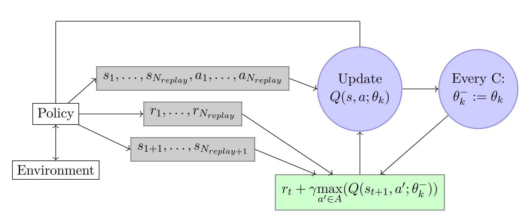
- Similar to fitted Q-learning, the target Q-network is: $$Y _ { k } ^ { Q } = r + \gamma \max _ { a ^ { \prime } \in \mathcal { A } } Q ( s ^ { \prime } , a ^ { \prime } ; \theta _ {k} ^ {-})$$ where $\theta _ { k } ^ { - }$ are updated only every $C \in \mathbb { N }$ iterations with the following assignment: $\theta _ { k } ^ { - } = \theta _ { k }$. This prevents the instabilities to propagate quickly and it reduces the risk of divergence as the target values $Y _ { k } ^ { Q }$ are kept fixed for $C$ iterations.
- In an online setting, the replay memory keeps all information for the last $N _ {replay} \in \mathbb{N}$ time steps. The updates are then made on a set of tuples $<s,a,r,s ^ {\prime} >$ (called mini-batch) selected randomly within the replay memory. This allows for updates that cover a wide range of the state-action space. In addition, one mini-batch update has less variance compared to a single tuple update.
- To keep the target values in a reasonable scale and to ensure proper learning in practice, rewards are clipped between -1 and +1. Clipping the rewards limits the scale of the error derivatives and makes it easier to use the same learning rate across multiple games (however, it introduces a bias).
Double DQN:
- The max operation in Q-learning uses the same values both to select and to evaluate an action. This makes it more likely to select overestimated values in case of inaccuracies or noise, resulting in overoptimistic value estimates. Therefore, the DQN algorithm induces an upward bias. The double estimator method uses two estimates for each variable, which allows for the selection of an estimator and its value to be uncoupled (Hasselt, 2010). This allows for the removal of the positive bias in estimating the action values.
- In Double DQN, or DDQN, the target value $Y _ {k} ^ {Q}$ is replaced by: $$Y _ {k} ^ {DDQN} = r + \gamma Q ( s ^ { \prime } , \underset { a \in \mathcal { A } } { \operatorname { argmax } } Q ( s ^ { \prime } , a ; \theta _ { k } ) ; \theta _ { k } ^ { - })$$ which leads to less overestimation of the Q-learning values, as well as improved stability, hence improved performance. Note that the policy is still chosen according to the values obtained by the current weights $\theta$.
- How about triple DQN or $N$ DQN? Possbile research project.

02/20: Deep Reinforcement Learning: Value-based methods for deep RL (3)

Dueling network architecture:
- The dueling network architecture decouples the value and advantage function $A ^ {\pi}(s, a)$. The Q-value function is given by: $$Q ( s , a ; \theta ^ { ( 1 ) } , \theta ^ { ( 2 ) } , \theta ^ { ( 3 ) } ) = V ( s ; \theta ^ { ( 1 ) } , \theta ^ { ( 3 ) } )+ ( A ( s , a ; \theta ^ { ( 1 ) } , \theta ^ { ( 2 ) } ) - \max _ { a ^ { \prime } \in \mathcal { A } } A ( s , a ^ { \prime } ; \theta ^ { ( 1 ) } , \theta ^ { ( 2 ) } ) )$$ (Question: why not just Q=V+A?)
  For $a ^ { * } = \operatorname { argmax } _ { a ^ { \prime } \in \mathcal { A } } Q ( s , a ^ { \prime } ; \theta ^ { ( 1 ) } , \theta ^ { ( 2 ) } , \theta ^ { ( 3 ) } )$, we have $Q ( s , a ^ { * } ; \theta ^ { ( 1 ) } , \theta ^ { ( 2 ) } , \theta ^ { ( 3 ) } ) = V ( s ; \theta ^ { ( 1 ) } , \theta ^ { ( 3 ) } )$.
- The structure of dueling network:
  
  The stream $V( s ; \theta ^ { ( 1 ) } , \theta ^ { ( 3 ) })$ provides an estimate of the value function, while the other stream produces an estimate of the advantage function. The learning update is done as in DQN and it is only the structure of the neural network that is modiﬁed.
- A slightly different approach is preferred in practice because it increases the stability of the optimization: $$Q ( s , a ; \theta ^ { ( 1 ) } , \theta ^ { ( 2 ) } , \theta ^ { ( 3 ) } ) = V ( s ; \theta ^ { ( 1 ) } , \theta ^ { ( 3 ) } ) + ( A ( s , a ; \theta ^ { ( 1 ) } , \theta ^ { ( 2 ) } ) - \frac { 1 } { | \mathcal { A } | } \sum _ { a ^ { \prime } \in \mathcal { A } } A ( s , a ^ { \prime } ; \theta ^ { ( 1 ) } , \theta ^ { ( 2 ) } ) )$$ In that case, the advantages only need to change as fast as the mean, which appears to work better in practice.
Distributional DQN:
- Another approach is to aim for a richer representation through a value distribution, i.e. the distribution of possible cumulative returns. This value distribution provides more complete information of the intrinsic randomness of the rewards and transitions of the agent within its environment (note that it is not a measure of the agent’s uncertainty about the environment).
- The value distribution $Z ^ {\pi}$ is a mapping from state-action pairs to distributions of returns when following policy $\pi$. It has an expectation equal to $Q ^ {\pi}$: $$Q ^ { \pi } ( s , a ) = \mathbb { E } [ Z ^ { \pi } ( s , a ) ]$$ This random return is also described by a recursive equation:
  $$Z ^ { \pi } ( s , a ) = R ( s , a , S ^ { \prime } ) + \gamma Z ^ { \pi } ( S ^ { \prime } , A ^ { \prime } )$$ where we use capital letters to emphasize the random nature of the next state-action pair $(S ^ {\prime}, A ^ {\prime})$ and $A ^ { \prime } \sim \pi ( \cdot | S ^ { \prime } )$.
- This approach has two main advantages: 1. It is possible to implement risk-aware behavior. 2. It leads to more performant learning in practice. The distributional perspective naturally provides a richer set of training signals than a scalar value function $Q(s,a)$. These training signals that are not a priori necessary for optimizing the expected return are known as auxiliary tasks and lead to an improved learning.

02/21: Deep Reinforcement Learning: Value-based methods for deep RL (4)

Multi-step learning:
- Non-bootstrapping methods learn directly from returns (Monte Carlo) and an intermediate solution is to use a multi-step target. Such a variant in the case of DQN can be obtained by using the n-step target value given by: $$Y _ { k } ^ { Q , n } = \sum _ { t = 0 } ^ { n - 1 } \gamma ^ { t } r _ { t } + \gamma ^ { n } \max _ { a ^ { \prime } \in A } Q ( s _ { n } , a ^ { \prime } ; \theta _ { k } )$$ where $( s _ { 0 } , a _ { 0 } , r _ { 0 } , \cdots , s _ { n - 1 } , a _ { n - 1 } , r _ { n - 1 } , s _ { n })$ is any trajectory of $n+1$ time steps with $s = s _ 0$ and $a = a _ 0$.
- A combination of different multi-steps targets can also be used: $$Y _ { k } ^ { Q , n } = \sum _ { i = 0 } ^ { n - 1 } \lambda _ { i } ( \sum _ { t = 0 } ^ { i } \gamma ^ { t } r _ { t } + \gamma ^ { i + 1 } \max _ { a ^ { \prime } \in A } Q ( s _ { i + 1 } , a ^ { \prime } ; \theta _ { k } ) )$$ with $\sum _ { i = 0 } ^ { n - 1 } \lambda _ { i } = 1$. In the method called TD($\lambda$), $n \rightarrow \infty$ and $\lambda _ { i }$ follow a geometric law: $\lambda _ { i } \propto \lambda ^ { i }$ where $0 \leq \lambda \leq 1$.
Bootstrapping:
- Disadvantage: using pure bootstrapping methods (such as in DQN) are prone to instabilities when combined with function approximation because they make recursive use of their own value estimate at the next time-step. Methods that rely less on bootstrapping can propagate information more quickly from delayed rewards as they learn directly from returns.
- Advantage: using value bootstrap allows learning from off-policy samples. With bootstrapping, most algorithms learn faster.

02/22: Possible RL Project: Maxmin learning with approximation

The basic idea for this project is combining double learning with approximation. As mentioned in Rich’s book, many algorithms involve a maximization operation which leads to maximization bias. By using double learning technique, the selection of an estimator and its value is uncoupled. Thus, we can remove the maximization bias to some extent. For example, for double Q-learning, the update is

$$Q _ { 1 } ( S _ { t } , A _ { t } ) \leftarrow Q _ { 1 } ( S _ { t } , A _ { t } ) + \alpha [ R _ { t + 1 } + \gamma Q _ { 2 } ( S _ { t + 1 } , \underset { a } { \arg \max } Q _ { 1 } ( S _ { t + 1 } , a ) ) - Q _ { 1 } ( S _ { t } , A _ { t } ) ]$$

A comparison of Q-learning and double Q-learning on a simple episodic MDP:

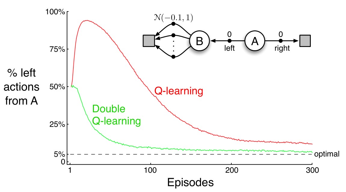
As shown in the above picture, double Q-learning is less affected by maximization bias. However, there is still a small gap between the optimal and what double Q-learning really archieves. Why is that? I think the main reason is that although the selection of an estimator and its value is uncoupled, the maximization operation still induces bias.

To address this problem, I come up with a new algorithm called maxmin Q-learning. Compared with double Q-learning, there are two important difference.

There are $n$ Q functions $Q _ 1, \cdots, Q _ n$where $n \in \mathbb{N}$ instead of just 2.
The update is consists of two steps:
- First, compute $Q _ {min} (s, a) = min(Q _ 1(s, a), \cdots, Q _ n(s, a))$.
- With probability $\frac{1}{n}$, update one of Q functions, say $Q _ 1$: $Q _ { 1 } ( S _ { t } , A _ { t } ) \leftarrow Q _ { 1 } ( S _ { t } , A _ { t } ) + \alpha [ R _ { t + 1 } + \gamma Q _ { min } ( S _ { t + 1 } , \underset { a } { \arg \max } Q _ { min } ( S _ { t + 1 } , a ) ) - Q _ { 1 } ( S _ { t } , A _ { t } ) ]$

For tabular case, maxmin Q-learning is better than double Q-learning on a simple episodic MDP. And it archieves the optimal!

I want to further test this algorithm in function approximation case. To be specific, I want to check if it can still mitigate maximization bias and compare the performance of between maxmin Q-learning and double Q-learning.

Moreover, since we have $n$ Q functions, can we apply ideas in Adaboost to get a better (with less bias) estimation of Q value?

02/25: Deep Reinforcement Learning: Policy gradient methods (1)

Stochastic Policy Gradient

The expected return of a stochastic policy $\pi$ starting from a given state $s _ 0$: $$V ^ { \pi } \left( s _ { 0 } \right) = \int _ { \mathcal { S } } \rho ^ { \pi } ( s ) \int _ { \mathcal { A } } \pi ( s , a ) R ^ { \prime } ( s , a ) da ds$$ where $R^{\prime}(s, a)=\int_{s^{\prime} \in \mathcal{S}} \operatorname{Pr}\left(s, a, s^{\prime}\right) R\left(s, a, s^{\prime}\right)$ and $\rho \pi (s)$ is the discounted state distribution defined as: $$\rho ^ { \pi } ( s ) = \sum _ { t = 0 } ^ { \infty } \gamma ^ { t } \operatorname {Pr} ( s _ { t } = s | s _ { 0 } , \pi )$$
For a differentiable policy $\pi _ w$, the fundamental result underlying these algorithms is the policy gradient theorem: $$\nabla _ { w } V ^ { \pi _ { w } } \left( s _ { 0 } \right) = \int _ { \mathcal { S } } \rho ^ { \pi _ { w } } ( s ) \int _ { \mathcal { A } } \nabla _ { w } \pi _ { w } ( s , a ) Q ^ { \pi _ { w } } ( s , a ) da ds$$ This result allows us to adapt the policy parameters from experience. This result is particularly interesting since the policy gradient does not depend on the gradient of the state distribution (even though one might have expected it to). The REINFORCE algorithm is a simple example.
Policy gradient methods should include two steps:
- Policy evaluation: estimates $Q ^ { \pi _ { w } }$.
- Policy improvement: it takes a gradient step to optimize the policy $\pi _ w(s, a)$ with respect to the value function estimation. Intuitively, the policy improvement step increases the probability of the actions proportionally to their expected return.
How to obtain an estimate of $Q ^ { \pi _ { w } }$?
- Monte-Carlo policy gradient: it estimates the $Q ^ { \pi _ { w } } (s,a)$ from rollouts on the environment while following policy $\pi _ { w }$. It is unbiased and, without instabilities induced by bootstrapping. However, the estimate requires on-policy rollouts and can exhibit high variance. Several rollouts are typically needed to obtain a good estimate of the return (not sample efficient).
- Actor-critic methods: use an estimate of the return given by a value-based approach, more efficient.
Remarks:
- To prevent the policy from becoming deterministic, it is common to add an entropy regularizer to the gradient. With this regularizer, the learnt policy can remain stochastic. This ensures that the policy keeps exploring.
- Advantage value function: While $Q ^ { \pi _ { w } } (s,a)$ summarizes the performance of each action for a given state under policy $\pi _ w$, the advantage function $A ^ { \pi _ { w } } (s,a)$ provides a measure of comparison for each action to the expected return at the state $s$, given by $V ^ { \pi _ { w } } (s)$. Using $A ^ { \pi _ { w } } ( s , a ) = Q ^ { \pi _ { w } } ( s , a ) - V ^ { \pi _ { w } } ( s )$ has usually lower magnitudes than $Q ^ { \pi _ { w } } (s,a)$. This helps reduce the variance of the gradient estimator in the policy improvement step, while not modifying the expectation. The value function $V ^ {{ \pi } _ w} ( s )$ can be seen as a baseline or control variate for the gradient estimator. Using such a baseline allows for improved numerical efficiency – i.e. reaching a given performance with fewer updates – because the learning rate can be bigger.

02/26: Deep Reinforcement Learning: Policy gradient methods (2)

Deterministic Policy Gradient

Let us denote by $\pi (s)$ the deterministic policy: $\pi ( s ) : \mathcal { S } \rightarrow \mathcal { A }$. In discrete action spaces, a direct approach is to build the policy iteratively with: $$\pi _ { k + 1 } ( s ) = \underset { a \in \mathcal { A } } { \operatorname { argmax } } Q ^ { \pi _ { k } } ( s , a )$$ where $\pi _ { k }$ is the policy at the $k$th iteration.
Deep Deterministic Policy Gradient (DDPG): In continuous action spaces, a greedy policy improvement becomes problematic, requiring a global maximization at every step. Instead, let us denote by $\pi _ w ( s )$ a differentiable deterministic policy. In that case, a simple and computationally attractive alternative is to move the policy in the direction of the gradient of $Q$: $$\nabla _ { w } V ^ { \pi _ { w } } \left( s _ { 0 } \right) = \mathbb { E } _ { s \sim \rho ^ { \pi _ { w } } } \left[ \nabla _ { w } \left( \pi _ { w } \right) \nabla _ { a } \left. \left( Q ^ { \pi _ { w } } ( s , a ) \right) \right| _ { a = \pi _ { w } ( s ) } \right]$$ This equation implies relying on $\nabla _ { a } \left( Q ^ { \pi w } ( s , a ) \right)$ (in addition to $\nabla _ { a } \left( Q ^ { \pi w } ( s , a ) \right)$), which usually requires using actor-critic methods.

02/27: Deep Reinforcement Learning: Policy gradient methods (3)

Actor-Critic Methods

The actor refers to the policy and the critic to the estimate of a value function (e.g., the Q-value function). In deep RL, both the actor and the critic can be represented by non-linear neural network function approximators. The actor uses gradients derived from the policy gradient theorem and adjusts the policy parameters $w$. The critic, parameterized by $\theta$, estimates the approximate value function for the current policy $\pi$.

The critic:
- TD(0): at every iteration, the current value $Q(s,a;\theta)$ is updated towards a target value: $Y _ { k } ^ { Q } = r + \gamma Q \left( s ^ { \prime } , a = \pi \left( s ^ { \prime } \right) ; \theta \right)$. It is simple yet not computationally efficient as it uses a pure bootstrapping technique that is prone to instabilities and has a slow reward propagation backwards in time.
- Retrace ($\lambda$): (i) it can make use of samples collected from any behavior policy without introducing a bias and (ii) it is efficient as it makes the best use of samples collected from near on-policy behavior policies. These architectures are sample-efficient thanks to the use of a replay memory, and computationally efficient since they use multi-step returns which improves the stability of learning and increases the speed of reward propagation backwards in time.
The actor: the off-policy gradient in the policy improvement phase for the stochastic case is given as: $$\nabla _ { w } V ^ { \pi _ { w } } \left( s _ { 0 } \right) = \mathbb { E } _ { s \sim \rho ^ { \pi _ { \beta } } , a \sim \pi _ { \beta } } \left[ \nabla _ { \theta } \left( \log \pi _ { w } ( s , a ) \right) Q ^ { \pi _ { w } } ( s , a ) \right]$$ where $\beta$ is a behavior policy generally different than $\pi$, which makes the gradient generally biased.
- In the case of actor-critic methods, an approach to perform the policy gradient on-policy without experience replay has been investigated with the use of asynchronous methods, where multiple agents are executed in parallel and the actor-learners are trained asynchronously. The parallelization of agents also ensures that each agent experiences different parts of the environment at a given time step. In that case, n-step returns can be used without introducing a bias. It removes the need to maintain a replay buffer. However, it is not sample efficient.
- An alternative is to combine off-policy and on-policy samples to trade-off both the sample efficiency of off-policy methods and the stability of on-policy gradient estimates. For example, Q-Prop uses a Monte Carlo on-policy gradient estimator, while reducing the variance of the gradient estimator by using an off-policy critic as a control variate. One limitation of Q-Prop is that it requires using on-policy samples for estimating the policy gradient.

02/28: Deep Reinforcement Learning: Policy gradient methods (4)

Natural Policy Gradients

Natural policy gradient methods use the steepest direction given by the Fisher information metric, i.e. the update follows the direction that maximizes $( J ( w ) - J ( w + \Delta w ) )$ under a constraint on $| \Delta w | _ { 2 }$.
In the hypothesis that the constraint on $\Delta w$ is defined with another metric than $L _ 2$, the first-order solution to the constrained optimization problem typically has the form $\Delta w \propto B ^ { - 1 } \nabla _ { w } J ( w )$ where B is an $n _ w \times n _ w$ matrix.
In natural gradients, the norm uses the Fisher information metric, given by a local quadratic approximation to the KL divergence $D _ {KL} \left( \pi ^ { w } | \pi ^ { w + \Delta w } \right)$. The natural gradient ascent for improving the policy π w is given by： $$\Delta w \propto F _ { w } ^ { - 1 } \nabla _ { w } V ^ { \pi _ { w } } ( \cdot )$$ where $F _ { w }$ is the Fisher information matrix given by: $$F _ { w } = \mathbb { E } _ { \pi _ { w } } \left[ \nabla _ { w } \log \pi _ { w } ( s , \cdot ) \left( \nabla _ { w } \log \pi _ { w } ( s , \cdot ) \right) ^ { T } \right]$$
As the angle between natural and ordinary gradient is never larger than ninety degrees, convergence is also guaranteed when using natural gradients. In the case of neural networks and their large number of parameters, it is usually impractical to compute, invert, and store the Fisher information matrix.

Trust Region Optimization

The policy optimization methods based on trust region restrict the changes in a policy using the KL divergence between the action distributions. By bounding the size of the policy update, trust region methods also bound the changes in state distributions guaranteeing improvements in policy.
Trust Region Policy Optimization (TRPO): uses constrained updates and advantage function estimation to perform the update, resulting in the reformulated optimization given by $$\max _ { \Delta w } \mathbb { E } _ { s \sim \rho ^ { \pi } w , a \sim \pi } \left[ \frac { \pi _ { w + \Delta w } ( s , a ) } { \pi _ { w } ( s , a ) } A ^ { \pi _ w } ( s , a ) \right]$$ subject to $\mathbb { E }[ D _ { \mathrm { KL } } \left( \pi _ { w } ( s , \cdot ) | \pi _ { w + \Delta w } ( s , \cdot ) \right) ] \leq \delta$, where $\delta \in \mathbb{R}$ is a hyperparameter.
Proximal Policy Optimization (PPO): it is a variant of the TRPO algorithm, which formulates the constraint as a penalty or a clipping objective, instead of using the KL constraint. PPO considers modifying the objective function to penalize changes to the policy that move r t ( w ) = π w+4w (s,a) π w (s,a) away from 1. The clipping objective that PPO maximizes is given by: $$\underset { s \sim \rho ^ { \pi } w , a \sim \pi _ { w } } { \mathbb { E } } \left[ \min \left( r _ { t } ( w ) A ^ { \pi _ { w } } ( s , a ) , \operatorname { clip } \left( r _ { t } ( w ) , 1 - \epsilon , 1 + \epsilon \right) A ^ { \pi _ { w } } ( s , a ) \right) \right]$$ where $\epsilon \in \mathbb{R}$ is a hyperparameter. This objective function clips the probability ratio to constrain the changes of $r _ t$ in the interval $[1− \epsilon, 1+ \epsilon]$.

March

03/01: Deep Reinforcement Learning: Policy gradient methods (5)

Combining policy gradient and Q-learning

Policy gradient algorithms have the following properties unlike the methods based on DQN:
- They are able to work with continuous action spaces. This is particularly interesting in applications such as robotics, where forces and torques can take a continuum of values.
- They can represent stochastic policies, which is useful for building policies that can explicitly explore. This is also useful in settings where the optimal policy is a stochastic policy (e.g., in a multi-agent setting where the Nash equilibrium is a stochastic policy).
Combine policy gradient methods directly with off-policy Q-learning: In some specific settings, depending on the loss function and the entropy regularization used, value-based methods and policy-based methods are equivalent. For instance, when adding an entropy regularization, we have: $$\nabla _ { w } V ^ { \pi _ { w } } \left( s _ { 0 } \right) = \mathbb { E } _ { s , a } \left[ \nabla _ { w } \left( \log \pi _ { w } ( s , a ) \right) Q ^ { \pi _ { w } } ( s , a ) \right] + \alpha \mathbb { E } _ { s } [ \nabla _ { w } H ^ { \pi _ { w } } ( s )]$$ where $H ^ { \pi } ( s ) = - \sum _ { a } \pi ( s , a ) \log \pi ( s , a )$. From this, one can note that an optimum is satisfied by the following policy: $\pi _ { w } ( s , a ) = \exp ( \frac{A ^ { \pi _ w } ( s , a )}{\alpha} - H ^ { \pi _ w } ( s ) )$. Therefore, we can use the policy to derive an estimate of the advantage function: $$\tilde { A } ^ { \pi _ { w } } ( s , a ) = \alpha \left( \log \pi _ { w } ( s , a ) + H ^ { \pi } ( s ) \right)$$
Both value-based and policy-based methods are model-free and they do not make use of any model of the environment.

03/02: Deep Reinforcement Learning: Model-based methods (1)

Pure model-based methods: When a model of the environment is available, planning consists in interacting with the model to recommend an action. In the case of discrete actions, lookahead search is usually done by generating potential trajectories. In the case of a continuous action space, trajectory optimization with a variety of controllers can be used.

Lookahead search: limited to discrete actions
- A lookahead search in an MDP iteratively builds a decision tree where the current state is the root node. It stores the obtained returns in the nodes and focuses attention on promising potential trajectories.
- Monte-Carlo tree search (MCTS): The idea is to sample multiple trajectories from the current state until a terminal condition is reached (e.g., a given maximum depth). From those simulation steps, the MCTS algorithm then recommends an action to take.
- Recent works have developed strategies to directly learn end-to-end the model, along with how to make the best use of it, without relying on explicit tree search techniques. These approaches show improved sample eﬃciency, performance, and robustness to model misspeciﬁcation compared to the separated approach (simply learning the model and then relying on it during planning). Why?
Trajectory optimization:
- If the model is differentiable, one can directly compute an analytic policy gradient by backpropagation of rewards along trajectories. For instance, PILCO uses Gaussian processes to learn a probabilistic model of the dynamics. It can then explicitly use the uncertainty for planning and policy evaluation in order to achieve a good sample efficiency. However, the gaussian processes have not been able to scale reliably to high-dimensional problems.
- Wahlström et al. (2015) uses a deep learning model of the dynamics (with an auto-encoder) along with a model in a latent state space. Model-predictive control (Morari and Lee, 1999) can then be used to find the policy by repeatedly solving a finite-horizon optimal control problem in the latent space.
- Watter et al. (2015) builds a probabilistic generative model in a latent space with the objective that it possesses a locally linear dynamics, which allows control to be performed more efficiently.
- Another approach is to use the trajectory optimizer as a teacher rather than a demonstrator: guided policy search takes a few sequences of actions suggested by another controller. It then learns to adjust the policy from these sequences.

03/03: Deep Reinforcement Learning: Model-based methods (2)

Integrating model-free and model-based methods: the respective strengths of the model-free versus model-based approaches depend on different factors.

The best suited approach depends on whether the agent has access to a model of the environment. If that’s not the case, the learned model usually has some inaccuracies that should be taken into account.
A model-based approach requires working in conjunction with a planning algorithm (or controller), which is often computationally demanding. The time constraints for computing the policy $\pi (s)$ via planning must therefore be taken into account (e.g., for applications with real-time decision-making or simply due to resource limitations).
For some tasks, the structure of the policy (or value function) is the easiest one to learn, but for other tasks, the model of the environment may be learned more efficiently due to the particular structure of the task (less complex or with more regularity). Thus, the most performant approach depends on the structure of the model, policy, and value function.

How to obtain advantages from both worlds by integrating learning and planning:

When the model is available, one direct approach is to use tree search techniques that make use of both value and policy networks.
When the model is not available and under the assumption that the agent has only access to a limited number of trajectories, the key property is to have an algorithm that generalizes well. One possibility is to build a model that is used to generate additional samples for a model-free reinforcement learning algorithm. Another possibility is to use a model-based approach along with a controller such as MPC to perform basic tasks and use model-free fine-tuning in order to achieve task success.
Other approaches build neural network architectures that combine both model-free and model-based elements. The VIN architecture (Tamar et al., 2016) is a fully differentiable neural network with a planning module that learns to plan from model-free objectives (given by a value function). It works well for tasks that involve planning-based reasoning (navigation tasks) from one initial position to one goal position and it demonstrates strong generalization in a few different domains.

Improving the combination of model-free and model-based ideas is one key area of research for the future development of deep RL algorithms.

03/04: Deep Reinforcement Learning: Generalization (1)

Generalization refers to either

the capacity to achieve good performance in an environment where limited data has been gathered, or
the capacity to obtain good performance in a related environment.

In the former case, the idea of generalization is directly related to the notion of sample efficiency (e.g., when the state-action space is too large to be fully visited). In the latter case, the test environment has common patterns with the training environment but can differ in the dynamics and the rewards. For instance, the underlying dynamics may be the same but a transformation on the observations may have happened.

Let us consider the case of a finite dataset $D$ obtained on the exact same task as the test environment. Formally, a dataset available to the agent $D \sim D$ can be defined as a set of four-tuples $(s, a, r, s^{\prime}) \in S \times A \times R \times S$ gathered by sampling independently and identically (i.i.d.).

a given number of state-action pairs $(s,a)$ from some fixed distribution with $P(s, a)>0$, $\forall (s,a) \in S \times A$;
a next state $s ^ {\prime} \sim P(s, a, \cdot)$;
a reward $r = R(s, a, s ^ {\prime})$; We denote by $D _ {\infty}$ the particular case of a dataset $D$ where the number of tuples tends to infinity.

A learning algorithm can be seen as a mapping of a dataset $D$ into a policy $\pi _ D$. Then we can decompose the suboptimality of the expected return as follows:

$$\underset { D \sim \mathcal { D } } { \mathbb { E } } [ V ^ { \pi ^ { * } } ( s ) - V ^ { \pi _ { D } } ( s ) ]$$ $$= \underset { D \sim \mathcal { D } } { \mathbb { E } } [ V ^ { \pi ^ { * } } ( s ) - V ^ { \pi _ { D \infty } } ( s ) + V ^ { \pi _ { D \infty } ( s ) } - V ^ { \pi _ { D } } ( s ) ]$$ $$ = \underbrace { ( V ^ { \pi ^ { * } } ( s ) - {V ^ { \pi _ { D _ { \infty } } } ( s ) ) } } _ { \text {asymptotic bias} } + \underbrace { \underset { D \sim \mathcal { D } } { \mathbb { E } } [ { V ^ { \pi _ { D \infty } } ( s ) } - V ^ { \pi _ { D } } ( s ) ] } _ { \text {error due to finite size of the dataset } D } $$

This decomposition highlights two different terms: (i) an asymptotic bias which is independent of the quantity of data and (ii) an overfitting term directly related to the fact that the amount of data is limited.

Improving generalization can be seen as a tradeoff between (i) an error due to the fact that the algorithm trusts completely the frequentist assumption (i.e., discards any uncertainty on the limited data distribution) and (ii) an error due to the bias introduced to reduce the risk of overfitting. When the quality of the dataset is low, the learning algorithm should favor more robust policies (i.e., consider a smaller class of policies with stronger generalization capabilities). When the quality of the dataset increases, the risk of overﬁtting is lower and the learning algorithm can trust the data more, hence reducing the asymptotic bias.

03/05: Deep Reinforcement Learning: Generalization (2)

We discuss the following key elements that are at stake when one wants to improve generalization in deep RL:

the state representation;
the learning algorithm (type of function approximator, model-free vs model-based);
the objective function (e.g., reward shaping, tuning the training discount factor);
using hierarchical learning.

Different aspects that can be used to avoid overfitting to limited data.

Feature selection: The appropriate level of abstraction plays a key role in the bias-overﬁtting tradeoﬀ and one of the key advantages of using a small but rich abstract representation is to allow for improved generalization.
- Overfitting: When considering many features on which to base the policy, an RL algorithm may take into consideration spurious correlations, which leads to overfitting.
- Asymptotic bias: Removing features that discriminate states with a very different role in the dynamics introduces an asymptotic bias. The same policy would be enforced on undistinguishable states, hence leading to a sub-optimal policy.
- In deep RL, one approach is to ﬁrst infer a factorized set of generative factors from the observations. This can be done for instance with an encoder-decoder architecture variant. These features can then be used as inputs to a reinforcement learning algorithm. The learned representation can, in some contexts, greatly help for generalization as it provides a more succinct representation that is less prone to overfitting. Some features may be kept in the abstract representation because they are important for the reconstruction of the observations, though they are otherwise irrelevant for the task at hand. Crucial information about the scene may also be discarded in the latent representation, particularly if that information takes up a small proportion of the observations $x$ in pixel space.
Learning algorithm and function approximator selection:
- If the function approximator used for the value function and/or the policy and/or the model is too simple, an asymptotic bias may appear. When the function approximator has poor generalization, there will be a large error due to the finite size of the dataset (overfitting).
- One approach to mitigate non-informative features is to force the agent to acquire a set of symbolic rules adapted to the task and to reason on a more abstract level. This abstract level reasoning and the improved generalization have the potential to induce high-level cognitive functions such as transfer learning and analogical reasoning. For instance, the function approximator may embed a relational learning structure and thus build on the idea of relational reinforcement learning.
- Auxiliary tasks: In the context of deep reinforcement learning, Jaderberg et al. (2016) show that augmenting a deep reinforcement learning agent with auxiliary tasks within a jointly learned representation can drastically improve sample efficiency in learning. This is done by maximizing simultaneously many pseudo-reward functions. The argument is that learning related tasks introduces an inductive bias that causes a model to build features in the neural network that are useful for the range of tasks. By explicitly learning both the model-free and model-based components through the state representation, along with an approximate entropy maximization penalty, the CRAR agent (François-Lavet et al., 2018) shows how it is possible to learn a low-dimensional representation of the task. In addition, this approach can directly make use of a combination of model-free and model-based, with planning happening in a smaller latent state space.

03/06: Deep Reinforcement Learning: Generalization (3)

Modifying the objective function

In order to improve the policy learned by a deep RL algorithm, one can optimize an objective function that diverts from the actual objective. By doing so, a bias is usually introduced but this can in some cases help with generalization.

Reward shaping: In practice, reward shaping uses prior knowledge by giving intermediate rewards for actions that lead to desired outcome. It is usually formalized as a function $F(s, a, s ^ {\prime})$ added to the original reward function $R(s, a, s ^ {\prime})$ of the original MDP. This technique is often used in deep reinforcement learning to improve the learning process in settings with sparse and delayed rewards.
Discount factor:
- When the model available to the agent is estimated from data, the policy found using a shorter planning horizon can actually be better than a policy learned with the true horizon. On the one hand, artiﬁcially reducing the planning horizon leads to a bias since the objective function is modified. However, if a long planning horizon is targeted (the discount factor $\gamma$ is close to 1), there is a higher risk of overfitting. This can intuitively be understood as linked to the accumulation of the errors in the transitions and rewards estimated from data as compared to the actual transition and reward probabilities.
- A high discount factor also requires specific care in value iteration algorithms as it can lead to instabilities in convergence. This effect is due to the mappings used in the value iteration algorithms with bootstrapping that propagate errors more strongly with a high discount factor. When bootstrapping is used in a deep RL value iteration algorithm, the risk of instabilities and overestimation of the value function is empirically stronger for a discount factor close to one.

03/11: Deep Reinforcement Learning: Generalization (4)

Hierarchical learning: The possibility of learning temporally extended actions (as opposed to atomic actions that last for one time-step) has been formalized under the name of options. The usage of options is an important challenge in RL because it is essential when the task at hand requires working on long time scales while developing generalization capabilities and easier transfer learning between the strategies.

Bias-overfitting tradeoff: For a given algorithmic parameter setting and keeping all other things equal, the right level of complexity is the one at which the increase in bias is equivalent to the reduction of overfitting (or the increase in overfitting is equivalent to the reduction of bias).

Offline setting:
- Regression-based approach: fit an MDP model to the data via regression (or simply use the frequentist statistics for finite state and action space). The empirical MDP can then be used to evaluate the policy. This purely model-based estimator has alternatives that do not require fitting a model. One possibility is to use a policy evaluation step obtained by generating artificial trajectories from the data, without explicitly referring to a model, thus designing a Model-free Monte Carlo-like (MFMC) estimator.
- Importance sampling approach: use the idea of importance sampling that lets us obtain an estimate of $V ^ { \pi } ( s )$ from trajectories that come from a behavior policy $\beta \neq \pi$ , where $\beta$ is assumed to be known. That approach is unbiased but the variance usually grows exponentially in horizon, which renders the method unsuitable when the amount of data is low.
- Mix of the regression-based approach and the importance sampling approach: use a doubly-robust estimator that is both unbiased and with a lower variance than the importance sampling estimators.
Online setting: A performant policy from given data is part of the solution to an efficient exploration/exploitation tradeoff. For that reason, progressively fitting a function approximator as more data becomes available can in fact be understood as a way to obtain a good bias-overfitting tradeoff throughout learning. With the same logic, progressively increasing the discount factor allows optimizing the bias-overfitting tradeoff through learning. Besides, optimizing the bias-overfitting tradeoff also suggests the possibility to dynamically adapt the feature space and/or the function approximator.

03/12: Deep Reinforcement Learning: Challenges in the online setting (1)

In the online setting, two specific elements have not yet been discussed in depth. First, the agent can influence how to gather experience so that it is the most useful for learning. Second, the agent has the possibility to use a replay memory that allows for a good data-efficiency.

Exploration/Exploitation dilemma: Exploration is about obtaining information about the environment (transition model and reward function) while exploitation is about maximizing the expected return given the current knowledge. As an agent starts accumulating knowledge about its environment, it has to make a tradeoff between learning more about its environment (exploration) or pursuing what seems to be the most promising strategy with the experience gathered so far (exploitation).

Different settings in the exploration/exploitation dilemma:
- First setting: The agent is expected to perform well without a separate training phase. Thus, an explicit tradeoff between exploration versus exploitation appears so that the agent should explore only when the learning opportunities are valuable enough for the future to compensate what direct exploitation can provide. The sub-optimality $\underset { s _ { 0 } } { \mathbb { E } } [ V ^ { * } ( s _ { 0 } ) - V ^ { \pi } ( s _ { 0 } ) ]$ of an algorithm obtained in this context is known as the cumulative regret.
- Common setting: The agent is allowed to follow a training policy during a ﬁrst phase of interactions with the environment so as to accumulate training data and hence learn a test policy. In the training phase, exploration is only constrained by the interactions it can make with the environment (e.g., a given number of interactions). The test policy should then be able to maximize a cumulative sum of rewards in a separate phase of interaction. The sub-optimality $\underset { s _ { 0 } } { \mathbb { E } } [ V ^ { * } ( s _ { 0 } ) - V ^ { \pi } ( s _ { 0 } ) ]$ obtained in this case of setting is known as the simple regret. Note that an implicit exploration/exploitation is still important. The agent has to ensure that the lesser-known parts of the environment are not promising (exploration). And the agent is interested in gathering experience in the most promising parts of the environment (which relates to exploitation) to reﬁne the knowledge of the dynamics.
Approaches to exploration:
- Directed exploration: The agent makes use of a memory of the past interactions with the environment. For MDPs, directed exploration can scale polynomially with the size of the state space while undirected exploration scales in general exponentially with the size of the state space. Inspired by the Bayesian setting, directed exploration can be done via heuristics of exploration bonus or by maximizing Shannon information gains. The key challenge for directed exploration is to handle, for high-dimensional spaces, the exploration/exploitation tradeoff in a principled way – with the idea to encourage the exploration of the environment where the uncertainty due to limited data is the highest. When rewards are not sparse, a measure of the uncertainty on the value function can be used to drive the exploration. When rewards are sparse, this is even more challenging and exploration should in addition be driven by some novelty measures on the observations (or states in a Markov setting).
- Undirected exploration: The agent does not rely on any exploration specific knowledge of the environment, such as $\epsilon$-greedy and softmax exploration (also called Boltzmann exploration) which takes an action with a probability that depends on the associated expected return.

03/13: Deep Reinforcement Learning: Challenges in the online setting (2)

Managing experience replay

In online learning, the agent has the possibility to use a replay memory that allows for data-efficiency by storing the past experience of the agent in order to have the opportunity to reprocess it later. In addition, a replay memory also ensures that the mini-batch updates are done from a reasonably stable data distribution kept in the replay memory which helps for convergence/stability. In an online setting, the replay memory keeps all information for the last $N _{replay} \in N$ time steps, where $N _{replay}$ is constrained by the amount of memory available.
While a replay memory allows processing the transitions in a different order than they are experienced, there is also the possibility to use prioritized replay. This allows for consideration of the transitions with a different frequency than they are experienced depending on their significance (that could be which experience to store and which ones to replay). A disadvantage of prioritized replay is that, in general, it also introduces a bias; indeed, by modifying the apparent probabilities of transitions and rewards, the expected return gets biased. Note that this bias can be partly or completely corrected using weighted importance sampling, and this correction is important near convergence at the end of training.

03/14: Deep Reinforcement Learning: Beyond MDPs (1)

Partial observability and the distribution of (related) MDPs: In both two settings, at each step in the sequential decision process, the agent may beneﬁt from taking into account its whole observable history up to the current time step $t$ when deciding what action to perform. In other words, a history of observations can be used as a pseudo-state (pseudo-state because that refers to a diﬀerent and abstract stochastic control process). Any missing information in the history of observations (potentially long before time $t$) can introduce a bias in the RL algorithm.

The partially observable scenario

Partially Observable Markov Decision Process (POMDP): A POMDP is a 7-tuple ($S, A, T, R, \Omega, O, \gamma$) where:
- $S$ is a finite set of states ${1, \cdots , N _ S}$,
- $A$ is a finite set of actions ${1, \cdots , N _ A}$,
- $P: S \times A \times S \rightarrow [0, 1]$ is the transition function,
- $R: S \times A \times S \rightarrow R$ is the reward function, where $R$ is a continuous set of possible rewards in a range $R _ {max} \in R ^ {+}$,
- $\Omega$ is a ﬁnite set of observations ${1, \cdots , N _ {\Omega}}$,
- $O: S \times \Omega \rightarrow [0, 1]$ is a set of conditional observation probabilities,
- $\gamma \in [0,1)$ is the discount factor.
The environment starts in a distribution of initial states $b(s _ 0)$. At each time step $t \in \mathbb{N} _ {0}$, the environment is in a state $s _ {t} \in S$. At the same time, the agent receives an observation $\omega _ {t} \in \Omega$ that depends on the state of the environment with probability $O(s _ {t}, {\omega} _ {t})$, after which the agent chooses an action $a _ {t} \in A$. Then, the environment transitions to state $s _ {t+1} \in S$ with probability $P(s _ {t}, a _ {t}, s _ {t+1})$ and the agent receives a reward $r _ {t} \in R$ equal to $R(s _ {t}, a _ {t}, s _ {t+1})$.
When the full model ($P$, $R$ and $O$) are known, methods such as Point-Based Value Iteration (PBVI) algorithm for POMDP planning can be used to solve the problem.
We denote by $H _ { t } = \Omega \times ( A \times R \times \Omega ) ^ { t }$ the set of histories observed up to time $t$ for $t \in {N _ 0}$, and by $H = \bigcup _ { t = 0 } ^ { \infty } H _ { t }$ the space of all possible observable histories.

Architectures such as convolutional layers or recurrency are particularly well-suited to deal with a large input space because they offer interesting generalization properties. A few empirical successes on large scale POMDPs make use of convolutional layers and/or recurrent layers, such as LSTMs.

03/15: Deep Reinforcement Learning: Beyond MDPs (2)

The distribution of (related) environments

In this setting, the environment of the agent is a distribution of different (yet related) tasks that differ for instance in the reward function or in the probabilities of transitions from one state to another. Each task $T _ {i} \sim T$ can be defined by the observations $\omega _ {t} \in \Omega$ (which are equal to $s _ {t}$ if the environments are Markov), the rewards $r _ {t} \in R$, as well as the effect of the actions $a _ {t} \in A$ taken at each step. Similarly to the partially observable context, we denote the history of observations by $H _ {t}$, where $H _ { t } \in H _ { t } = \Omega \times ( A \times R \times \Omega ) ^ { t }$. The agent aims at finding a policy $\pi ( a _ { t } | H _ { t } ; \theta )$ with the objective of maximizing its expected return, defined (in the discounted setting) as $$\underset { T _ { i } \sim \mathcal { T } } { \mathbb { E } } [ \sum _ { k = 0 } ^ { \infty } \gamma ^ { k } r _ { t + k } | H _ { t } , \pi ]$$
Different approaches have been investigated in the literature. The Bayesian approach aims at explicitly modeling the distribution of the different environments, if a prior is available. However, it is often intractable to compute the Bayesian-optimal strategy and one has to rely on more practical approaches that do not require an explicit model of the distribution. The concept of meta-learning or learning to learn aims at discovering, from experience, how to behave in a range of tasks and how to negotiate the exploration-exploitation tradeoff. Some other approaches have also been investigated. One possibility is to train a neural network to imitate the behavior of known optimal policies on MDPs drawn from the distribution. The parameters of the model can also be explicitly trained such that a small number of gradient steps in a new task from the distribution will produce fast learning on that task.

03/18: Deep Reinforcement Learning: Beyond MDPs (3)

Transfer learning

Zero-shot learning: The idea of zero-shot learning is that an agent should be able to act appropriately in a new task directly from experience acquired on other similar tasks. To achieve this, the agent must either (i) develop generalization capacities described or (ii) use speciﬁc transfer strategies that explicitly retrain or replace some of its components to adjust to new tasks. The underlying reason for these successes is the ability of the deep learning architecture to generalize between states that have similar high-level representations and should therefore have the same value function/policy in diﬀerent domains. Another approach to zero-shot transfer is to use algorithms that enforce states that relate to the same underlying task but have diﬀerent renderings to be mapped into an abstract state that is close. To develop generalization capacities, one approach is to use an idea similar to data augmentation in supervised learning so as to make sense of variations that were not encountered in the training data.
Lifelong learning or continual learning: lifelong machine learning relates to the capability of a system to learn many tasks over a lifetime from one or more domains. In general, deep learning architectures can generalize knowledge across multiple tasks by sharing network parameters. A direct approach is thus to train function approximators (e.g. policy, value function, model, etc.) sequentially in diﬀerent environments. The difficulty of this approach is to ﬁnd methods that enable the agent to retain knowledge in order to more efficiently learn new tasks. The problem of retaining knowledge in deep reinforcement learning is complicated by the phenomenon of catastrophic forgetting, where generalization to previously seen data is lost at later stages of learning. The straightforward approach is to either (i) use experience replay from all previous experience, or (ii) retrain occasionally on previous tasks similar to the meta-learning setting. When these two options are not available, or as a complement to the two previous approaches, one can use deep learning techniques that are robust to forgetting, such as progressive networks. The idea is to leverage prior knowledge by adding, for each new task, lateral connections to previously learned features (that are kept fixed). Other approaches to limiting catastrophic forgetting include slowing down learning on the weights important for previous tasks and decomposing learning into skill hierarchies.
Curriculum learning: the goal of curriculum learning is to explicitly design a sequence of source tasks for an agent to train on such that the ﬁnal performance or learning speed is improved on a target task. The idea is to start by learning small and easy aspects of the target task and then to gradually increase the difficulty level.

03/19: Deep Reinforcement Learning: Beyond MDPs (4)

Learning without explicit reward function (1)

Due to the complexity of environments in practical applications, deﬁning a reward function can turn out to be rather complicated. There are two other possibilities: (i) given demonstrations of the desired task, we can use imitation learning or extract a reward function using inverse reinforcement learning; (ii) a human may provide feedback on the agent’s behavior in order to deﬁne the task.

Learning from demonstrations: Given an observed behavior (e.g. the trajectories of an expert/teacher agent), the goal is to have the agent perform similarly. Two approaches are possible:
- Imitation learning uses supervised learning to map states to actions from the observations of the expert’s behavior.
- Inverse reinforcement learning (IRL) determines a possible reward function given observations of optimal behavior. For example, let us consider a large MDP for which the expert always ends up transitioning to the same state. In that context, one may be able to easily infer, from only a few trajectories, what the probable goal of the task is (a reward function that explains the behavior of the teacher), as opposed to directly learning the policy via imitation learning, which is much less efficient.
- Another setting requires the agent to learn directly from a sequence of observations without corresponding actions (and possibly in a slightly different context). This may be done in a meta-learning setting by providing positive reward to the agent when it performs as it is expected based on the demonstration of the teacher. The agent can then act based on new unseen trajectories of the teacher, with the objective that is can generalize sufficiently well to perform new tasks.

03/20: Deep Reinforcement Learning: Beyond MDPs (5)

Learning without explicit reward function (2)

Learning from direct feedback: Learning from feedback investigates how an agent can interactively learn behaviors from a human teacher who provides positive and negative feedback signals. In order to learn complex behavior, human trainer feedbacks has the potential to be more performant than a reward function deﬁned a priori.
Multi-agent systems:
- A multi-agent POMDP with $N$ agents is a tuple ($S, A _ { N }, \ldots , A _ { N } , P , R _ { 1 } , \ldots , R _ { N } , \Omega , O _ { 1 } , \ldots , O _ { N } , \gamma$) where:
- S is a finite set of states {$1, \ldots, N _ {S}$} (describing the possible configurations of all agents);
- $A = A _ {1} \times \ldots \times A _ {n}$ is a finite set of actions {$1, \ldots , N _ {A}$};
- $P : S \times A \times S \rightarrow [0, 1]$ is the transition function (set of conditional transition probabilities between states);
- $\forall i , R _ { i } : S \times A _ { i } \times S \rightarrow \mathbb{R}$ is the reward function for agent $i$;
- $\Omega$ is a finite set of observations {$1, \ldots, N _ {\Omega}$};
- $\forall i , O _ { i } : S \times \Omega \rightarrow [0, 1]$ is a set of conditional observation probabilities
- $\gamma \in [0, 1)$ is the discount factor.
- Collaborative versus non-collaborative setting: In a pure collaborative setting, agents have a shared reward measurement ($R _ {i} = R _ {j}, \forall i, j \in [1, \ldots, N]$). In a mixed or non-collaborative (possibly adversarial) setting each agent obtains different rewards. In both cases, each agent $i$ aims to maximize a discounted sum of its rewards $\sum _ { t = 0 } ^ { H } \gamma ^ { t } r _ { t } ^ { ( i ) }$.
- Decentralized versus centralized setting: In a decentralized setting, each agent selects its own action conditioned only on its local information. When collaboration is beneficial, this decentralized setting can lead to the emergence of communication between agents in order to share information. In a centralized setting, the RL algorithm has access to all observations $w ^ {(i)}$ and all rewards $r ^ {(i)}$. The problem can be reduced to a single-agent RL problem on the condition that a single objective can be defined (in a purely collaborative setting, the unique objective is straightforward). Note that even when a centralized approach can be considered (depending on the problem), an architecture that does not make use of the multi-agent structure usually leads to sub-optimal learning.
In general, multi-agent systems are challenging because agents are independently updating their policies as learning progresses, and therefore the environment appears non-stationary to any particular agent. For training one particular agent, one approach is to select randomly the policies of all other agents from a pool of previously learned policies. This can stabilize training of the agent that is learning and prevent overfitting to the current policy of the other agents.

03/21: Deep Reinforcement Learning: Perspectives on deep reinforcement learning (1)

Challenges of applying reinforcement learning to real-world problems: In practice, even in the case where the task is well deﬁned (explicit reward function), there is one fundamental difficulty: it is often not possible to let an agent interact freely and sufficiently in the actual environment (or set of environments), due to either safety, cost or time constraints.

The agent may not be able to interact with the true environment but only with an inaccurate simulation of it. When ﬁrst learning in a simulation, the diﬀerence with the real-world domain is known as the reality gap.
The acquisition of new observations may not be possible anymore (e.g. the batch setting). This scenario happens for instance in medical trials, in tasks with dependence on weather conditions or in trading markets (e.g. energy markets and stock markets).

In order to deal with these limitations, different elements are important:

One can aim to develop a simulator that is as accurate as possible.
One can design the learning algorithm so as to improve generalization and/or use transfer learning methods.

03/22: Deep Reinforcement Learning: Perspectives on deep reinforcement learning (2)

Relations between deep RL and neuroscience

During the development of algorithms able to solve challenging sequential decision-making tasks, biological plausibility was not a requirement from an engineering standpoint. However, biological intelligence has been a key inspiration for many of the most successful algorithms.

Reinforcement: Driven by such connections, many aspects of reinforcement learning have also been investigated directly to explain certain phenomena in the brain. For instance, computational models have been an inspiration to explain cognitive phenomena such as exploration and temporal discounting of rewards. In cognitive science, Kahneman has also described that there is a dichotomy between two modes of thoughts: a “System 1” that is fast and instinctive and a “System 2” that is slower and more logical. In deep reinforcement, a similar dichotomy can be observed when we consider the model-free and the model-based approaches. Indeed, a conscious thought at a particular time instant can be seen as a low-dimensional combination of a few concepts in order to take decisions.
Deep learning: Deep learning also finds its origin in models of neural processing in the brain of biological entities. However, subsequent developments are such that deep learning has become partly incompatible with current knowledge of neurobiology. The convolutional structure used in deep learning that is inspired by the organization of the animal visual cortex.

03/25: Lifelong Learning [Introduction]: Definition of LL (1)

Lifelong learning (LL) is a continuous learning process. At any point in time, the learner has performed a sequence of $N$ learning tasks, $T _ { 1 } , T _ { 2 } , \ldots , T _ { N }$. These tasks have their corresponding datasets $D _ { 1 } , D _ { 2 } , \ldots , D _ { N }$. The tasks can be of different types and from different domains. When faced with the ($N+1$)th task $T _ {N+1}$ (the new or current task) with its data $D _ {N+1}$, the learner can leverage the past knowledge in the knowledge base (KB) to help learn $T _ {N+1}$. The task may be given or discovered by the system itself. The objective of LL is usually to optimize the performance of the new task $T _ {N+1}$, but it can optimize any task by treating the rest of the tasks as the previous tasks. KB maintains the knowledge learned and accumulated from learning the previous tasks. After the completion of learning $T _ {N+1}$, KB is updated with the knowledge gained from learning $T _ {N+1}$. The updating can involve consistency checking, reasoning, and meta-mining of higher-level knowledge. Ideally, an LL learner should also be able to:

learn and function in the open environment, where it not only can apply the learned model or knowledge to solve problems but also discover new tasks to be learned.
learn to improve the model performance in the application or testing of the learned model.

Remarks:

Five key characteristics of LL:
1. continuous learning process,
2. knowledge accumulation and maintenance in the KB,
3. the ability to use the accumulated past knowledge to help future learning,
4. the ability to discover new tasks,
5. the ability to learn while working or to learn on the job.
Knowledge, in fact, plays a central rule. It not only can help improve future learning, but can also help collect and label training data (self-supervision)and discover new tasks to be learned in order to achieve autonomy in learning. The integration of both data-driven learning and knowledge-driven learning is probably what human learning is all about.
The shift to the new task can happen abruptly or gradually, and the tasks and their data do not have to be provided by some external systems or human users. Ideally, a lifelong learner should also be able to find its own learning tasks and training data in its interaction with humans and the environment or using its previously learned knowledge to perform open-world and self-supervised learning.
The definition indicates that LL may require a systems approach that combines multiple learning algorithms and diﬀerent knowledge representation schemes. It is unlikely that a single learning algorithm is able to achieve the goal of LL.

03/26: Lifelong Learning [Introduction]: Definition of LL (2)

Knowledge Base (KB): It is mainly for storing the previously learned knowledge. It has a few sub-components.

Past Information Store(PIS)：It stores the information resulted from the past learning. PIS may involve sub-stores for information such as (1) the original data used in each previous task, (2) intermediate results from each previous task, and (3) the final model or patterns learned from each previous task.
Meta-Knowledge Miner (MKM): It performs meta-mining of the knowledge in the PIS and in the meta-knowledge store. The resulting knowledge is stored in the Meta-Knowledge Store. Here multiple mining algorithms may be used to produce diﬀerent types of results.
Meta-Knowledge Store (MKS): It stores the knowledge mined or consolidated from PIS and also from MKS itself. Some suitable knowledge representation schemes are needed for each application.
Knowledge Reasoner (KR): It makes inference based on the knowledge in MKB and PIS to generate more knowledge. With the advance of LL, this component will become increasingly important.

Knowledge-Based Learner (KBL): For LL, it is necessary for the learner to be able to use prior knowledge in learning. We call such a learner a knowledge-based learner, which can leverage the knowledge in the KB to learn the new task. This component may have two sub-components:

Task knowledge miner (TKM), which makes use of the raw knowledge or information in the KB to mine or identify knowledge that is appropriate for the current task. This is needed because in some cases, KBL cannot use the raw knowledge in the KB directly but needs some task-specific and more general knowledge mined from the KB.
The learner that can make use of the mined knowledge in learning.

Task-based Knowledge Miner (TKM): This module mines knowledge from the KB speciﬁcally for the new task.

Model: This is the learned model, which can be a prediction model or classiﬁer in supervised learning, clusters or topics in unsupervised learning, a policy in reinforcement learning, etc.

Application: This is the real-world application for the model. It is important to note that during model application, the system can still learn new knowledge, and possibly discover new tasks to be learned. Application can also give feedback to the knowledge-based learner for model improvement.

Task Manager (TM): It receives and manages the tasks that arrive in the system, handles the task shift, and presents the new learning task to the KBL in a lifelong manner.

Lifelong Learning Process: A typical LL process starts with the Task Manager assigning a new task to the KBL (the task can be given or discovered automatically). KBL then works with the help of the past knowledge stored in the KB to produce an output model for the user and also send the information or knowledge that needs to be retained for future use to the KB. In the application process, the system may also discover new tasks and learn while working (learn on the job). Some knowledge gained in applications can also be retained to help future learning.

03/27: Lifelong Learning [Introduction]: Types of Knowledge and Key Challenges

There is still no well-accepted definition of knowledge or its general representation scheme. In the current LL research, past knowledge usually serves as some kind of prior information (e.g., prior model parameters or prior probabilities) for the new task. For a particular LL algorithm and a particular form of shared knowledge, one needs to design a KB and its maintenance or updating methods based on the algorithm and its knowledge representation need. There are mainly two types of shared knowledge that are used in learning the new task.

Global knowledge: Many existing LL methods assume that there is a global latent structure among tasks that is shared by all tasks. This global structure can be learned and leveraged in the new task learning. The approaches based on global knowledge transfer and sharing mainly grew out of or inspired by MTL, which jointly optimizes the learning of multiple similar tasks. Such knowledge is more suitable for similar tasks in the same domain because such tasks are often highly correlated or have very similar distributions.
Local knowledge: Different tasks may use different pieces of knowledge learned from different previous tasks. We call such pieces of knowledge the local knowledge because they are local to their individual previous tasks and are not assumed to form a coherent global structure. Local knowledge is likely to be more suitable for related tasks from different domains because the shared knowledge from any two domains may be small. But the prior knowledge that can be leveraged by the new task can still be large because the prior knowledge can be from many past domains.

LL methods based on local knowledge usually focus on optimizing the current task performance with the help of past knowledge. They can also be used to improve the performance of any previous task by treating that task as the new/current task. The main advantage of these methods is their flexibility as they can choose whatever pieces of past knowledge that are useful to the new task. The main advantage of LL methods based on global knowledge is that they often approximate optimality on all tasks, including the previous and the current ones. This property is inherited from MTL. However, when the tasks are highly diverse and/or numerous, this can be difficult.

There are two other fundamental challenges about knowledge in LL:

Correctness of knowledge: In a nutshell, LL can be regarded as a continuous bootstrapping process. Errors can propagate from previous tasks to subsequent tasks to generate more and more errors. To deal with it, one strategy is to find those pieces of knowledge that have been discovered in many previous tasks/domains. Another strategy is to make sure that the piece of knowledge is discovered from different contexts using different techniques. However, two main issues remain. First, they are not foolproof because they can still produce wrong knowledge. Second, they have low recall because most pieces of correct knowledge cannot pass these strategies and thus cannot be used subsequently, which prevents LL from producing even better results.
Applicability of knowledge: Although a piece of knowledge may be correct in the context of some previous tasks, it may not be applicable to the current task.

03/27: Lifelong Learning [Introduction]: Evaluation Methodology and Role of Big Data

Experimental evaluation of an LL algorithm in the current research is commonly done using the following steps:

Run on the data from the previous tasks: We first run the algorithm on the data from a set of previous tasks, one at a time in a given sequence, and retain the knowledge gained in the KB.
Run on the data of the new task: We then run the LL algorithm on the new task data by leveraging the knowledge in the KB.
Run baseline algorithms: For comparison, we run some baseline algorithms. There are usually two kinds of baselines. The first kind are algorithms that perform isolated learning on the new data without using any past knowledge. The second kind are existing LL algorithms.
Analyze the results: This step compares the results from steps 2 and 3 and analyzes the results to make some observations, e.g., to show that the results from the LL algorithm in step 2 are superior to those from the baselines in step 3.

There are several additional considerations in carrying out an LL experimental evaluation.

A large number of tasks: A large number of tasks and datasets are needed to evaluate an LL algorithm. This is because the knowledge gained from a few tasks may not be able to improve the learning of the new task much as each task may only provide a very small amount of knowledge that is useful to the new task (unless all the tasks are very similar) and the data in the new task is often quite small.
Task sequence: The sequence of the tasks to be learned can be signiﬁcant, meaning that different task sequences can generate different results. This is so because LL algorithms typically do not guarantee optimal solutions for all previous tasks. To take the sequence effect into consideration in the experiment, one can try several random sequences of tasks and generate results for the sequences. The results can then be aggregated for comparison purposes.
Progressive experiments: Since more previous tasks generate more knowledge, and more knowledge in turn enables an LL algorithm to produce better results for the new task, it is thus desirable to show how the algorithm performs on the new task as the number of previous tasks increases.

Role of Big Data in LL Evaluation: It is important for an LL system to learn from a diverse range and a large number of domains to give the system a wide vocabulary and a wide range of knowledge so that it can help learn in diverse future domains. Furthermore, unlike transfer learning, LL needs to automatically identify the pieces of past knowledge that it can use, and not every past task/domain is useful to the current task. LL experiments and evaluation thus require data from a large number of domains or tasks and consequently large volumes of data.

03/28: Lifelong Learning [Lifelong Supervised Learning]: Lifelong Memory-Based Learning

Lifelong supervised learning is a continuous learning process where the learner has performed a sequence of $N$ supervised learning tasks, $T _ {1}, T _ {2}, \ldots , T _ {N}$, and retained the learned knowledge in a knowledge base. When a new task $T _ {N+1}$ arrives, the learner leverages the past knowledge in the KB to help learn a new model $f _ {N+1}$ from $T _ {N+1}$’s training data $D _ {N+1}$ After learning $T _ {N+1}$, the KB is also updated with the learned knowledge from $T _ {N+1}$.

Two Memory-Based learning methods:

K-Nearest Neighbors (KNN): Given a testing instance $x$, the algorithm finds $K$ examples in the training data $( x _ { i } , y _ { i })\in D$ whose feature vectors $x _ { i }$ are nearest to $x$ according to some distance metric such as the Euclidean distance. The predicted output is the mean value $\frac { 1 } { K } \sum y _ { i }$ of these nearest neighbors.
Shepard’s method: This method uses all the training examples in $D$ and weights each example according to the inverse distance to the test instance $x$: $$s ( x ) = ( \sum _ {(x _ {i} , y _ {i}) \in D } \frac { y _ { i } } { | x - x _ { i } | + \epsilon } ) \times ( \sum _ { (x _ { i } , y _ { i }) \in D } \frac{1}{| x - x _ { i } | + \epsilon}) ^ {-1}$$ where $\epsilon > 0$ is a small constant to avoid the denominator being zero. Neither KNN nor Shepard’s method can use the previous task data with different distributions or distinct class labels to help its classification.

Learning a new representation for LL:

Thrun proposed to learn a new representation to bridge the gap among tasks for the above two memory-based methods to achieve LL, which was shown to improve the predictive performance especially when the number of labeled examples is small.

Its goal is to learn a function $f: I \rightarrow {0,1}$ where $f(x)=1$ means that $x \in I$ belongs to a target concept (e.g., cat or dog); otherwise $x$ does not belong to the concept. For example, $f _ {dog} ( x ) = 1$ means that $x$ is an instance of the concept dog. Let the data from the previous $N$ tasks be $\mathcal { D } ^ { p } = { \mathcal { D } _ { 1 } , \mathcal { D } _ { 2 } , \ldots , \mathcal { D } _ { N } }$. Each past task data $\mathcal { D } _ { i } \in \mathcal { D } ^ { p }$ is associated with an unknown classification function $f _ {i}$. $\mathcal { D } ^ { p }$ is called the support set. The goal is to learn the function $f _ {N+1}$ for the current new task data $\mathcal{D} _ {N+1}$ with the help of the support set.

To bridge the difference among different tasks and to be able to exploit the shared information in the past data (the support set), the paper proposed to learn a new representation of the data, i.e., to learn a space transformation function $g : I \rightarrow I ^ { \prime }$ to map the original input feature vectors in $I$ to a new space $I ^ { \prime }$. The new space $I ^ { \prime }$ then serves as the input space for KNN or the Shepard’s method. The intuition is that positive examples of a concept (with $y=1$) should have similar new representations while a positive example and a negative example of a concept ($y=1$ and $y=0$) should have very different representations. This idea can be formulated as an energy function $E$ for $g$:

$$E = \sum _ { \mathcal { D } _ { i } \in \mathcal { D } ^ { p } } \sum _ { \langle x , y = 1 \rangle \in \mathcal { D } _ { i } } ( \sum _ { \langle x ^ { \prime } , y ^ { \prime } = 1 \rangle \in \mathcal { D } _ { i } } | g ( x ) - g ( x ^ { \prime } ) | - \sum _ { \langle x ^ { \prime } , y ^ { \prime } = 0 \rangle \in \mathcal { D } _ { i } } | g ( x ) - g ( x ^ { \prime } ) | )$$

The optimal function $g ^ {*}$ is achieved by minimizing the energy function $E$, which forces the distance between pairs of positive examples of the concept $(\langle x , y = 1 \rangle$ and $\langle x ^ { \prime } , y ^ { \prime } = 1 \rangle)$ to be small, and the distance between a positive example and a negative example of a concept $( \langle x , y = 1 \rangle$ and $\langle x ^ { \prime } , y ^ { \prime } = 0 \rangle)$ to be large.

Given the mapping function $g ^ { * }$, rather than performing memory-based learning in the original space $\langle x _ { i } , y _ { i } \rangle \in \mathcal { D } _ { N + 1 }$, $x _ {i}$ is first transformed to the new space using $g ^ {*}$ to $\langle g ^ { * } ( x _ { i } ) , y _ { i } \rangle$ before applying NN or the Shepard’s method.

03/29: Lifelong Learning [Lifelong Supervised Learning]: Lifelong Neural Networks

MTL Net: In MTL net, instead of building a neural network for each individual task, it constructs a universal neural network for all the tasks. This universal neural network uses the same input layer for input from all tasks and uses one output unit for each task (or class in this case). There is also a shared hidden layer in MTL net that is trained in parallel using Back-Propagation on all the tasks to minimize the error on all the tasks. This shared layer allows features developed for one task to be used by other tasks. For a specific task, it will activate some hidden units that are related to it while making the weights of the other irrelevant hidden units small. Essentially, like a normal batch MTL method, the system jointly optimizes the classification of all the past/previous and the current/new tasks.

Lifelong EBNN: EBNN (Explanation-Based Neural Network) is used for concept learning, which learns a function $f : I \rightarrow { 0,1 }$ to predict if an object represented by a feature vector $x \in I$ belongs to a concept ($y=1$) or not($y=0$).

In this approach, the system ﬁrst learns a general distance function, $d : I \times I \rightarrow [ 0,1 ]$, considering all the past data (or the support set) and uses this distance function to share or transfer the knowledge of the past task data to the new task $T _ {N+1}$. Given two input vectors, say $x$ and $y$, function d computes the probability of $x$ and $y$ being members of the same concept (or class), regardless what the concept is. The training data for learning the distance function is generated as follows: For each past task data $\mathcal { D } _ { i } \in \mathcal { D } ^ { p }$, each pair of examples of the concept generates a training example. For a pair, $\langle x , y = 1 \rangle \in \mathcal { D } _ { i }$ and $\left\langle x ^ { \prime } , y ^ { \prime } = 1 \right\rangle \in \mathcal { D } _ { i }$, a positive training example is generated, $\left\langle \left( x , x ^ { \prime } \right) , 1 \right\rangle$. For a pair $\langle x , y = 1 \rangle \in \mathcal { D } _ { i }$ and $\left\langle x ^ { \prime } , y ^ { \prime } = 0 \right\rangle \in \mathcal { D } _ { i }$ or $\langle x , y = 0 \rangle \in \mathcal { D } _ { i }$ and $\left\langle x ^ { \prime } , y ^ { \prime } = 1 \right\rangle \in \mathcal { D } _ { i }$, a negative training example is generated, $\left\langle \left( x , x ^ { \prime } \right) , 0 \right\rangle$.

Unlike a traditional neural network, EBNN estimates the slope (tangent) of the target function at each data point $x$ and adds it into the vector representation of the data point. In the new task $T _ {N+1}$, a training example is of the form, $\langle x , f _ { N + 1 } ( x ) , \nabla _ { x } f _ { N + 1 } ( x )\rangle$, where $f _ {N+1}(x)$ is just the original class label of $x \in D _ {N+1}$ (the new task data). The system is trained using Tangent-Prop algorithm. $\nabla _ {x} f _ {N+1}(x)$ is estimated using the gradient of the distance $d$ obtained from the neural network, i.e., $\nabla _ { x } f _ { N + 1 } ( x ) \approx \frac { \partial d _ { x ^ { \prime } } ( x ) } { \partial x }$, where $\left\langle x ^ { \prime } , y ^ { \prime } = 1 \right\rangle \in \mathcal { D } _ { N + 1 }$ and $d _ { x ^ { \prime } } ( x ) = d \left( x , x ^ { \prime } \right)$. The rationale is that the distance between $x$ and a positive training example $x ^ {\prime}$ is an estimate of the probability of $x$ being a positive example, which approximates $f _ {N+1} (x)$. As a result, the built EBNN fits both the current task data $\mathcal { D } _ { N + 1 }$ and the support set through $\nabla _ { x } f _ { N + 1 } ( x )$ and $d$.

Again, the knowledge base in EBNN stores only the past data. Similarly, this technique also does not deal with correctness or applicability of the shared knowledge $d$. It is also inefficient if the number of previous tasks is large because the training of the distance function d needs to be re-done using all the past data whenever a new task arrives. Additionally,since every pair of data points in each past task dataset forms a training example for learning the distance function d , the training data for learning $d$ can be huge.

Research Diary 2019

Reference

January

February

March