Introduction: Definition of LL

Lifelong learning (LL) is a continuous learning process. At any point in time, the learner has performed a sequence of $N$ learning tasks, $T _ { 1 } , T _ { 2 } , \ldots , T _ { N }$. These tasks have their corresponding datasets $D _ { 1 } , D _ { 2 } , \ldots , D _ { N }$. The tasks can be of different types and from different domains. When faced with the ($N+1$)th task $T _ {N+1}$ (the new or current task) with its data $D _ {N+1}$, the learner can leverage the past knowledge in the knowledge base (KB) to help learn $T _ {N+1}$. The task may be given or discovered by the system itself. The objective of LL is usually to optimize the performance of the new task $T _ {N+1}$, but it can optimize any task by treating the rest of the tasks as the previous tasks. KB maintains the knowledge learned and accumulated from learning the previous tasks. After the completion of learning $T _ {N+1}$, KB is updated with the knowledge gained from learning $T _ {N+1}$. The updating can involve consistency checking, reasoning, and meta-mining of higher-level knowledge. Ideally, an LL learner should also be able to:

learn and function in the open environment, where it not only can apply the learned model or knowledge to solve problems but also discover new tasks to be learned.
learn to improve the model performance in the application or testing of the learned model.

Remarks:

Five key characteristics of LL:
1. continuous learning process,
2. knowledge accumulation and maintenance in the KB,
3. the ability to use the accumulated past knowledge to help future learning,
4. the ability to discover new tasks,
5. the ability to learn while working or to learn on the job.
Knowledge, in fact, plays a central rule. It not only can help improve future learning, but can also help collect and label training data (self-supervision)and discover new tasks to be learned in order to achieve autonomy in learning. The integration of both data-driven learning and knowledge-driven learning is probably what human learning is all about.
The shift to the new task can happen abruptly or gradually, and the tasks and their data do not have to be provided by some external systems or human users. Ideally, a lifelong learner should also be able to find its own learning tasks and training data in its interaction with humans and the environment or using its previously learned knowledge to perform open-world and self-supervised learning.
The definition indicates that LL may require a systems approach that combines multiple learning algorithms and diﬀerent knowledge representation schemes. It is unlikely that a single learning algorithm is able to achieve the goal of LL.

Knowledge Base (KB): It is mainly for storing the previously learned knowledge. It has a few sub-components.

Past Information Store(PIS)：It stores the information resulted from the past learning. PIS may involve sub-stores for information such as (1) the original data used in each previous task, (2) intermediate results from each previous task, and (3) the final model or patterns learned from each previous task.
Meta-Knowledge Miner (MKM): It performs meta-mining of the knowledge in the PIS and in the meta-knowledge store. The resulting knowledge is stored in the Meta-Knowledge Store. Here multiple mining algorithms may be used to produce diﬀerent types of results.
Meta-Knowledge Store (MKS): It stores the knowledge mined or consolidated from PIS and also from MKS itself. Some suitable knowledge representation schemes are needed for each application.
Knowledge Reasoner (KR): It makes inference based on the knowledge in MKB and PIS to generate more knowledge. With the advance of LL, this component will become increasingly important.

Knowledge-Based Learner (KBL): For LL, it is necessary for the learner to be able to use prior knowledge in learning. We call such a learner a knowledge-based learner, which can leverage the knowledge in the KB to learn the new task. This component may have two sub-components:

Task knowledge miner (TKM), which makes use of the raw knowledge or information in the KB to mine or identify knowledge that is appropriate for the current task. This is needed because in some cases, KBL cannot use the raw knowledge in the KB directly but needs some task-specific and more general knowledge mined from the KB.
The learner that can make use of the mined knowledge in learning.

Task-based Knowledge Miner (TKM): This module mines knowledge from the KB speciﬁcally for the new task.

Model: This is the learned model, which can be a prediction model or classiﬁer in supervised learning, clusters or topics in unsupervised learning, a policy in reinforcement learning, etc.

Application: This is the real-world application for the model. It is important to note that during model application, the system can still learn new knowledge, and possibly discover new tasks to be learned. Application can also give feedback to the knowledge-based learner for model improvement.

Task Manager (TM): It receives and manages the tasks that arrive in the system, handles the task shift, and presents the new learning task to the KBL in a lifelong manner.

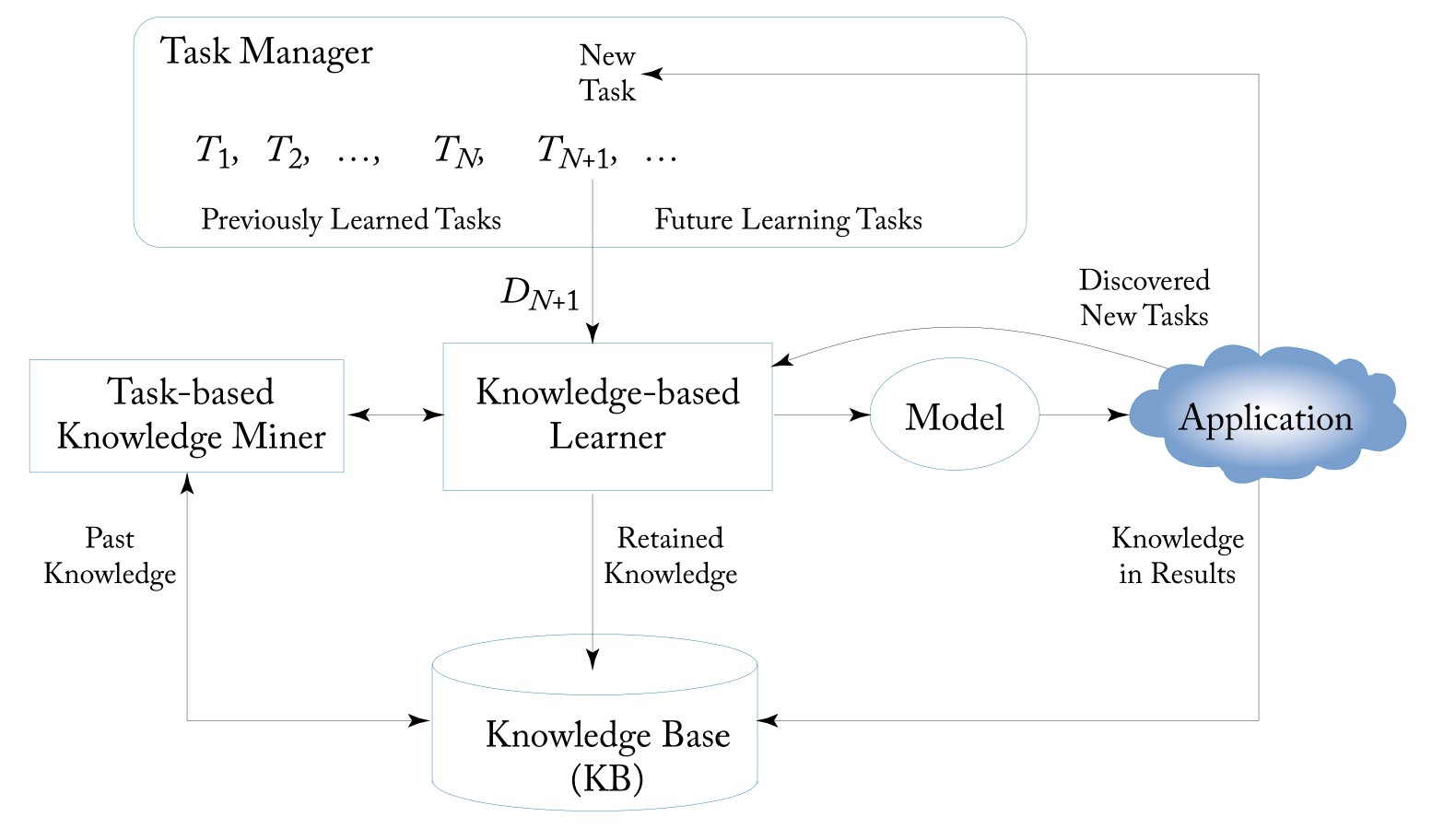
Lifelong Learning Process: A typical LL process starts with the Task Manager assigning a new task to the KBL (the task can be given or discovered automatically). KBL then works with the help of the past knowledge stored in the KB to produce an output model for the user and also send the information or knowledge that needs to be retained for future use to the KB. In the application process, the system may also discover new tasks and learn while working (learn on the job). Some knowledge gained in applications can also be retained to help future learning.

Introduction: Types of Knowledge and Key Challenges

There is still no well-accepted definition of knowledge or its general representation scheme. In the current LL research, past knowledge usually serves as some kind of prior information (e.g., prior model parameters or prior probabilities) for the new task. For a particular LL algorithm and a particular form of shared knowledge, one needs to design a KB and its maintenance or updating methods based on the algorithm and its knowledge representation need. There are mainly two types of shared knowledge that are used in learning the new task.

Global knowledge: Many existing LL methods assume that there is a global latent structure among tasks that is shared by all tasks. This global structure can be learned and leveraged in the new task learning. The approaches based on global knowledge transfer and sharing mainly grew out of or inspired by MTL, which jointly optimizes the learning of multiple similar tasks. Such knowledge is more suitable for similar tasks in the same domain because such tasks are often highly correlated or have very similar distributions.
Local knowledge: Different tasks may use different pieces of knowledge learned from different previous tasks. We call such pieces of knowledge the local knowledge because they are local to their individual previous tasks and are not assumed to form a coherent global structure. Local knowledge is likely to be more suitable for related tasks from different domains because the shared knowledge from any two domains may be small. But the prior knowledge that can be leveraged by the new task can still be large because the prior knowledge can be from many past domains.

LL methods based on local knowledge usually focus on optimizing the current task performance with the help of past knowledge. They can also be used to improve the performance of any previous task by treating that task as the new/current task. The main advantage of these methods is their flexibility as they can choose whatever pieces of past knowledge that are useful to the new task. The main advantage of LL methods based on global knowledge is that they often approximate optimality on all tasks, including the previous and the current ones. This property is inherited from MTL. However, when the tasks are highly diverse and/or numerous, this can be difficult.

There are two other fundamental challenges about knowledge in LL:

Correctness of knowledge: In a nutshell, LL can be regarded as a continuous bootstrapping process. Errors can propagate from previous tasks to subsequent tasks to generate more and more errors. To deal with it, one strategy is to find those pieces of knowledge that have been discovered in many previous tasks/domains. Another strategy is to make sure that the piece of knowledge is discovered from different contexts using different techniques. However, two main issues remain. First, they are not foolproof because they can still produce wrong knowledge. Second, they have low recall because most pieces of correct knowledge cannot pass these strategies and thus cannot be used subsequently, which prevents LL from producing even better results.
Applicability of knowledge: Although a piece of knowledge may be correct in the context of some previous tasks, it may not be applicable to the current task.

Introduction: Evaluation Methodology and Role of Big Data

Experimental evaluation of an LL algorithm in the current research is commonly done using the following steps:

Run on the data from the previous tasks: We first run the algorithm on the data from a set of previous tasks, one at a time in a given sequence, and retain the knowledge gained in the KB.
Run on the data of the new task: We then run the LL algorithm on the new task data by leveraging the knowledge in the KB.
Run baseline algorithms: For comparison, we run some baseline algorithms. There are usually two kinds of baselines. The first kind are algorithms that perform isolated learning on the new data without using any past knowledge. The second kind are existing LL algorithms.
Analyze the results: This step compares the results from steps 2 and 3 and analyzes the results to make some observations, e.g., to show that the results from the LL algorithm in step 2 are superior to those from the baselines in step 3.

There are several additional considerations in carrying out an LL experimental evaluation.

A large number of tasks: A large number of tasks and datasets are needed to evaluate an LL algorithm. This is because the knowledge gained from a few tasks may not be able to improve the learning of the new task much as each task may only provide a very small amount of knowledge that is useful to the new task (unless all the tasks are very similar) and the data in the new task is often quite small.
Task sequence: The sequence of the tasks to be learned can be signiﬁcant, meaning that different task sequences can generate different results. This is so because LL algorithms typically do not guarantee optimal solutions for all previous tasks. To take the sequence effect into consideration in the experiment, one can try several random sequences of tasks and generate results for the sequences. The results can then be aggregated for comparison purposes.
Progressive experiments: Since more previous tasks generate more knowledge, and more knowledge in turn enables an LL algorithm to produce better results for the new task, it is thus desirable to show how the algorithm performs on the new task as the number of previous tasks increases.

Role of Big Data in LL Evaluation: It is important for an LL system to learn from a diverse range and a large number of domains to give the system a wide vocabulary and a wide range of knowledge so that it can help learn in diverse future domains. Furthermore, unlike transfer learning, LL needs to automatically identify the pieces of past knowledge that it can use, and not every past task/domain is useful to the current task. LL experiments and evaluation thus require data from a large number of domains or tasks and consequently large volumes of data.

Lifelong Supervised Learning: Lifelong Memory-Based Learning

Lifelong supervised learning is a continuous learning process where the learner has performed a sequence of $N$ supervised learning tasks, $T _ {1}, T _ {2}, \ldots , T _ {N}$, and retained the learned knowledge in a knowledge base. When a new task $T _ {N+1}$ arrives, the learner leverages the past knowledge in the KB to help learn a new model $f _ {N+1}$ from $T _ {N+1}$’s training data $D _ {N+1}$ After learning $T _ {N+1}$, the KB is also updated with the learned knowledge from $T _ {N+1}$.

Two Memory-Based learning methods:

K-Nearest Neighbors (KNN): Given a testing instance $x$, the algorithm finds $K$ examples in the training data $( x _ { i } , y _ { i })\in D$ whose feature vectors $x _ { i }$ are nearest to $x$ according to some distance metric such as the Euclidean distance. The predicted output is the mean value $\frac { 1 } { K } \sum y _ { i }$ of these nearest neighbors.
Shepard’s method: This method uses all the training examples in $D$ and weights each example according to the inverse distance to the test instance $x$: $$s ( x ) = ( \sum _ {(x _ {i} , y _ {i}) \in D } \frac { y _ { i } } { | x - x _ { i } | + \epsilon } ) \times ( \sum _ { (x _ { i } , y _ { i }) \in D } \frac{1}{| x - x _ { i } | + \epsilon}) ^ {-1}$$ where $\epsilon > 0$ is a small constant to avoid the denominator being zero. Neither KNN nor Shepard’s method can use the previous task data with different distributions or distinct class labels to help its classification.

Learning a new representation for LL:

Thrun proposed to learn a new representation to bridge the gap among tasks for the above two memory-based methods to achieve LL, which was shown to improve the predictive performance especially when the number of labeled examples is small.

Its goal is to learn a function $f: I \rightarrow {0,1}$ where $f(x)=1$ means that $x \in I$ belongs to a target concept (e.g., cat or dog); otherwise $x$ does not belong to the concept. For example, $f _ {dog} ( x ) = 1$ means that $x$ is an instance of the concept dog. Let the data from the previous $N$ tasks be $\mathcal { D } ^ { p } = { \mathcal { D } _ { 1 } , \mathcal { D } _ { 2 } , \ldots , \mathcal { D } _ { N } }$. Each past task data $\mathcal { D } _ { i } \in \mathcal { D } ^ { p }$ is associated with an unknown classification function $f _ {i}$. $\mathcal { D } ^ { p }$ is called the support set. The goal is to learn the function $f _ {N+1}$ for the current new task data $\mathcal{D} _ {N+1}$ with the help of the support set.

To bridge the difference among different tasks and to be able to exploit the shared information in the past data (the support set), the paper proposed to learn a new representation of the data, i.e., to learn a space transformation function $g : I \rightarrow I ^ { \prime }$ to map the original input feature vectors in $I$ to a new space $I ^ { \prime }$. The new space $I ^ { \prime }$ then serves as the input space for KNN or the Shepard’s method. The intuition is that positive examples of a concept (with $y=1$) should have similar new representations while a positive example and a negative example of a concept ($y=1$ and $y=0$) should have very different representations. This idea can be formulated as an energy function $E$ for $g$:

$$E = \sum _ { \mathcal { D } _ { i } \in \mathcal { D } ^ { p } } \sum _ { \langle x , y = 1 \rangle \in \mathcal { D } _ { i } } ( \sum _ { \langle x ^ { \prime } , y ^ { \prime } = 1 \rangle \in \mathcal { D } _ { i } } | g ( x ) - g ( x ^ { \prime } ) | - \sum _ { \langle x ^ { \prime } , y ^ { \prime } = 0 \rangle \in \mathcal { D } _ { i } } | g ( x ) - g ( x ^ { \prime } ) | )$$

The optimal function $g ^ {*}$ is achieved by minimizing the energy function $E$, which forces the distance between pairs of positive examples of the concept $(\langle x , y = 1 \rangle$ and $\langle x ^ { \prime } , y ^ { \prime } = 1 \rangle)$ to be small, and the distance between a positive example and a negative example of a concept $( \langle x , y = 1 \rangle$ and $\langle x ^ { \prime } , y ^ { \prime } = 0 \rangle)$ to be large.

Given the mapping function $g ^ { * }$, rather than performing memory-based learning in the original space $\langle x _ { i } , y _ { i } \rangle \in \mathcal { D } _ { N + 1 }$, $x _ {i}$ is first transformed to the new space using $g ^ {*}$ to $\langle g ^ { * } ( x _ { i } ) , y _ { i } \rangle$ before applying NN or the Shepard’s method.

Lifelong Supervised Learning: Lifelong Neural Networks

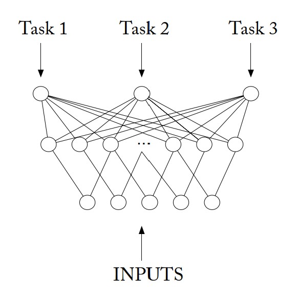
MTL Net: In MTL net, instead of building a neural network for each individual task, it constructs a universal neural network for all the tasks. This universal neural network uses the same input layer for input from all tasks and uses one output unit for each task (or class in this case). There is also a shared hidden layer in MTL net that is trained in parallel using Back-Propagation on all the tasks to minimize the error on all the tasks. This shared layer allows features developed for one task to be used by other tasks. For a specific task, it will activate some hidden units that are related to it while making the weights of the other irrelevant hidden units small. Essentially, like a normal batch MTL method, the system jointly optimizes the classification of all the past/previous and the current/new tasks.

Lifelong EBNN: EBNN (Explanation-Based Neural Network) is used for concept learning, which learns a function $f : I \rightarrow { 0,1 }$ to predict if an object represented by a feature vector $x \in I$ belongs to a concept ($y=1$) or not($y=0$).

In this approach, the system ﬁrst learns a general distance function, $d : I \times I \rightarrow [ 0,1 ]$, considering all the past data (or the support set) and uses this distance function to share or transfer the knowledge of the past task data to the new task $T _ {N+1}$. Given two input vectors, say $x$ and $y$, function d computes the probability of $x$ and $y$ being members of the same concept (or class), regardless what the concept is. The training data for learning the distance function is generated as follows: For each past task data $\mathcal { D } _ { i } \in \mathcal { D } ^ { p }$, each pair of examples of the concept generates a training example. For a pair, $\langle x , y = 1 \rangle \in \mathcal { D } _ { i }$ and $\left\langle x ^ { \prime } , y ^ { \prime } = 1 \right\rangle \in \mathcal { D } _ { i }$, a positive training example is generated, $\left\langle \left( x , x ^ { \prime } \right) , 1 \right\rangle$. For a pair $\langle x , y = 1 \rangle \in \mathcal { D } _ { i }$ and $\left\langle x ^ { \prime } , y ^ { \prime } = 0 \right\rangle \in \mathcal { D } _ { i }$ or $\langle x , y = 0 \rangle \in \mathcal { D } _ { i }$ and $\left\langle x ^ { \prime } , y ^ { \prime } = 1 \right\rangle \in \mathcal { D } _ { i }$, a negative training example is generated, $\left\langle \left( x , x ^ { \prime } \right) , 0 \right\rangle$.

Unlike a traditional neural network, EBNN estimates the slope (tangent) of the target function at each data point $x$ and adds it into the vector representation of the data point. In the new task $T _ {N+1}$, a training example is of the form, $\langle x , f _ { N + 1 } ( x ) , \nabla _ { x } f _ { N + 1 } ( x )\rangle$, where $f _ {N+1}(x)$ is just the original class label of $x \in D _ {N+1}$ (the new task data). The system is trained using Tangent-Prop algorithm. $\nabla _ {x} f _ {N+1}(x)$ is estimated using the gradient of the distance $d$ obtained from the neural network, i.e., $\nabla _ { x } f _ { N + 1 } ( x ) \approx \frac { \partial d _ { x ^ { \prime } } ( x ) } { \partial x }$, where $\left\langle x ^ { \prime } , y ^ { \prime } = 1 \right\rangle \in \mathcal { D } _ { N + 1 }$ and $d _ { x ^ { \prime } } ( x ) = d \left( x , x ^ { \prime } \right)$. The rationale is that the distance between $x$ and a positive training example $x ^ {\prime}$ is an estimate of the probability of $x$ being a positive example, which approximates $f _ {N+1} (x)$. As a result, the built EBNN fits both the current task data $\mathcal { D } _ { N + 1 }$ and the support set through $\nabla _ { x } f _ { N + 1 } ( x )$ and $d$.

Again, the knowledge base in EBNN stores only the past data. Similarly, this technique also does not deal with correctness or applicability of the shared knowledge $d$. It is also inefficient if the number of previous tasks is large because the training of the distance function d needs to be re-done using all the past data whenever a new task arrives. Additionally,since every pair of data points in each past task dataset forms a training example for learning the distance function d , the training data for learning $d$ can be huge.

Reference

Lifelong Machine Learning. Chen, Zhiyuan, and Bing Liu, 2016.